Why meteora?

While the API (and especially the underlying code) of meteora may appear rather abstract, the library serves a very simple purpose: making retrieving data from meteorological stations from different sources as easy as possible (or at least, this is what we intend).

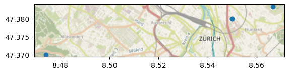
Let us illustrate the purpose of meteora with a very simple use case. Imagine you want to get meteorological observations for the Zurich (Switzerland) area. A good starting point is always the Global Historical Climatology Network hourly (GHCNh) dataset:

Show code cell source

Hide code cell source

import datetime as dt
import os
import types

import contextily as cx
import geopandas as gpd
import matplotlib.pyplot as plt
import numpy as np
import pandas as pd
import seaborn as sns
import xarray as xr
import xclim.indices as xci
from dask import diagnostics
from matplotlib import cm
from matplotlib import colors as mcolors

from meteora import clients, climate_indices, settings


# Suppress Dask progress bars used by the GHCNh client.
class _NoProgressBar:
    def __init__(self, *args, **kwargs):
        pass

    def __enter__(self):
        return self

    def __exit__(self, exc_type, exc, tb):
        return False

    def register(self):
        pass

    def unregister(self):
        pass


diagnostics.ProgressBar = _NoProgressBar


def _get_first_crs(client_dict):
    return list(client_dict.values())[0].CRS


def plot_single_axis(client_dict, *, crs=None, ax=None):
    """Plot stations from different clients in a single figure."""
    if crs is None:
        crs = _get_first_crs(client_dict)
    if ax is None:
        _, ax = plt.subplots()

    pd.concat(
        [
            client.stations_gdf.assign(source=client_label).to_crs(crs)
            for client_label, client in client_dict.items()
        ]
    ).plot("source", legend=True, ax=ax)
    cx.add_basemap(ax, crs=crs, attribution=False)

    return ax


def plot_multi_axes(client_dict, *, crs=None, col_wrap=2, colors=None):
    """Plot stations from different clients in a grid of subplots."""
    n_rows = len(client_dict) // col_wrap
    if crs is None:
        crs = _get_first_crs(client_dict)
    if len(client_dict) % col_wrap != 0:
        n_rows += 1
    if colors is None:
        colors = sns.color_palette()
    fig, axes = plt.subplots(
        nrows=n_rows,
        ncols=col_wrap,
        sharex=True,
        sharey=True,
        figsize=(col_wrap * figwidth, n_rows * figheight),
    )
    for (client_label, client), ax, color in zip(
        client_dict.items(), axes.flat, colors
    ):
        client.stations_gdf.to_crs(crs).plot(ax=ax, color=color)
        ax.set_title(client_label)

    xmin, xmax = np.inf, -np.inf
    ymin, ymax = np.inf, -np.inf
    for ax in axes.flat:
        xmin = min(xmin, ax.get_xlim()[0])
        xmax = max(xmax, ax.get_xlim()[1])
        ymin = min(ymin, ax.get_ylim()[0])
        ymax = max(ymax, ax.get_ylim()[1])

    for ax in axes.flat:
        ax.set_xlim(xmin, xmax)
        ax.set_ylim(ymin, ymax)
        cx.add_basemap(ax, crs=crs, attribution=False)

    return fig


def plot_ts_by_source(ts_df, variables, *, hue="source"):
    """Plot time series for multiple variables with a shared legend."""
    fig, axes = plt.subplots(
        ncols=len(variables),
        sharex=True,
        sharey=False,
        figsize=(2 * figwidth, figheight),
    )
    legend_flags = [False] * len(variables)
    if legend_flags:
        legend_flags[-1] = True
    plot_df = ts_df.reset_index()
    for variable, ax, legend in zip(variables, axes, legend_flags):
        sns.lineplot(plot_df, x="time", y=variable, hue=hue, ax=ax, legend=legend)
        ax.tick_params(axis="x", labelrotation=45)
    if legend_flags:
        sns.move_legend(axes[-1], "center left", bbox_to_anchor=(1.05, 0.5))
    fig.tight_layout()
    return fig


def get_seasonal_ts_df(client, start_year, end_year, start_month, end_month, variables):
    """Get multi-year seasonal time series data frame."""
    return pd.concat(
        [
            client.get_ts_df(
                variables,
                dt.date(year, start_month, 1),
                dt.datetime.combine(
                    dt.date(year, end_month + 1, 1) - dt.timedelta(days=1),
                    dt.time.max,
                ),
            )
            for year in range(start_year, end_year + 1)
        ],
        axis="rows",
    )


def plot_tn_facetgrid(
    tn_gdf,
    *,
    vmin=None,
    vmax=None,
    cmap=None,
    colorbar_label="N. tropical nights",
    **plot_kwargs,
):
    """Plot tropical nights in a FacetGrid with a shared colorbar."""
    with sns.axes_style("white"):
        g = sns.FacetGrid(tn_gdf, row="source", col="time")

    def _gdf_plot(data, **kwargs):
        _kwargs = kwargs.copy()
        _kwargs.pop("color", None)
        data.plot("tn", ax=plt.gca(), **_kwargs)

    g.map_dataframe(_gdf_plot, vmin=vmin, vmax=vmax, cmap=cmap, **plot_kwargs)

    for ax in g.axes.flat:
        cx.add_basemap(ax, crs=tn_gdf.crs, attribution=False)

    for ax in g.axes.flat:
        ax.axes.get_xaxis().set_visible(False)
        ax.axes.get_yaxis().set_ticks([])
        for spine in ["bottom", "left"]:
            ax.spines[spine].set_visible(False)

    g.set_titles(col_template="{col_name}", row_template="{row_name}")
    for ax_row in g.axes:
        ax_row[0].set_ylabel(ax_row[0].get_title().split(" | ")[0])
    for ax in g.axes[0]:
        ax.set_title(ax.get_title().split(" | ")[1])
    for ax_row in g.axes[1:]:
        for ax in ax_row:
            ax.set_title("")

    g.tight_layout()
    norm = mcolors.Normalize(vmin=vmin, vmax=vmax)
    sm = cm.ScalarMappable(norm=norm, cmap=cmap)
    cax = g.figure.add_axes([1, 0.3, 0.02, 0.4])
    g.figure.colorbar(sm, cax=cax, label=colorbar_label)

    return g

region = "Zurich, Switzerland"

netatmo_client_id = os.getenv("NETATMO_CLIENT_ID", default="")
netatmo_client_secret = os.getenv("NETATMO_CLIENT_SECRET", default="")
netatmo_stations_filepath = "data/zurich-netatmo-cws.gpkg"
era5_filepath = "data/8.34-47.28-8.67-47.54_era5_2m_temperature_m06-m08_2022-2024.nc"
crs = "epsg:4326"

# viz args
figwidth, figheight = plt.rcParams["figure.figsize"]
cmap = "coolwarm"

ghcnh_client = clients.GHCNHourlyClient(region)
ax = ghcnh_client.stations_gdf.plot()
cx.add_basemap(ax, crs=ghcnh_client.stations_gdf.crs, attribution=False)

(C) OpenStreetMap contributors, Tiles style by Humanitarian OpenStreetMap Team hosted by OpenStreetMap France

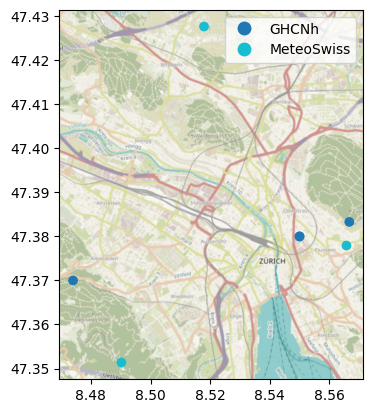
What if we wanted more stations? In this case, we could also try the Swiss Federal Office of Meteorology and Climatology (MeteoSwiss) via the MeteoSwissClient:

meteoswiss_client = clients.MeteoSwissClient(region)
_ = plot_single_axis({"GHCNh": ghcnh_client, "MeteoSwiss": meteoswiss_client})

(C) OpenStreetMap contributors, Tiles style by Humanitarian OpenStreetMap Team hosted by OpenStreetMap France

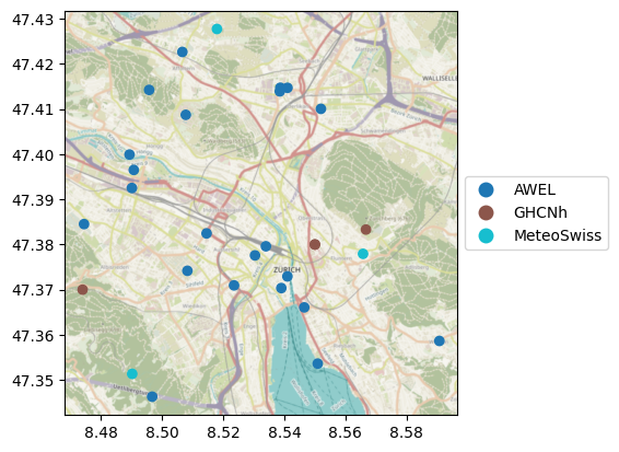
As we can see, using both clients improves the spatial density of the stations. What if we wanted even more? We can add the data from the Office for Waste, Water, Energy and Air (AWEL) of the canton of Zurich via the AWELClient:

awel_client = clients.AWELClient(region)
client_dict = {
    "GHCNh": ghcnh_client,
    "MeteoSwiss": meteoswiss_client,
    "AWEL": awel_client,
}
ax = plot_single_axis(
    client_dict,
)
sns.move_legend(ax, "center left", bbox_to_anchor=(1, 0.5))

(C) OpenStreetMap contributors, Tiles style by Humanitarian OpenStreetMap Team hosted by OpenStreetMap France

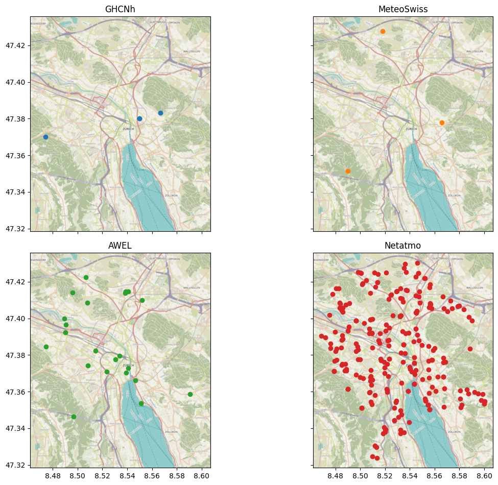
Can we still improve the spatial density of stations? In many cases, yes - enter citizen weather stations (CWS). Meteora features the NetatmoClient, which makes it easy to access public data from Netatmo weather stations (one of the major CWS providers). Let us focus on the city of Zurich:

use_netatmo_files = not netatmo_client_id or not netatmo_client_secret

if use_netatmo_files:
    # emulate the client `stations_gdf` attribute
    netatmo_client = types.SimpleNamespace(
        stations_gdf=gpd.read_file(netatmo_stations_filepath).set_index(
            settings.STATIONS_ID_COL
        )
    )
else:
    netatmo_client = clients.NetatmoClient(
        region, netatmo_client_id, netatmo_client_secret
    )

client_dict = {
    "GHCNh": ghcnh_client,
    "MeteoSwiss": meteoswiss_client,
    "AWEL": awel_client,
    "Netatmo": netatmo_client,
}

fig = plot_multi_axes(client_dict)
fig.tight_layout()

(C) OpenStreetMap contributors, Tiles style by Humanitarian OpenStreetMap Team hosted by OpenStreetMap France

As we can see, CWS can vastly improve the spatial density of weather observation, especially in urban areas of Europe and North America. Note that it is strongly recommended to quality-control (QC) CWS data before any climatological analysis - see a section dedicated to CWS QC with Meteora for more details on the subject.

To sum up: despite great standardization efforts of global climatological datasets such as GHCNh, there can be many other sources of meteorological data. The central objective of meteora is to provide a standardized API and data representation format for meteorological stations data in Python.

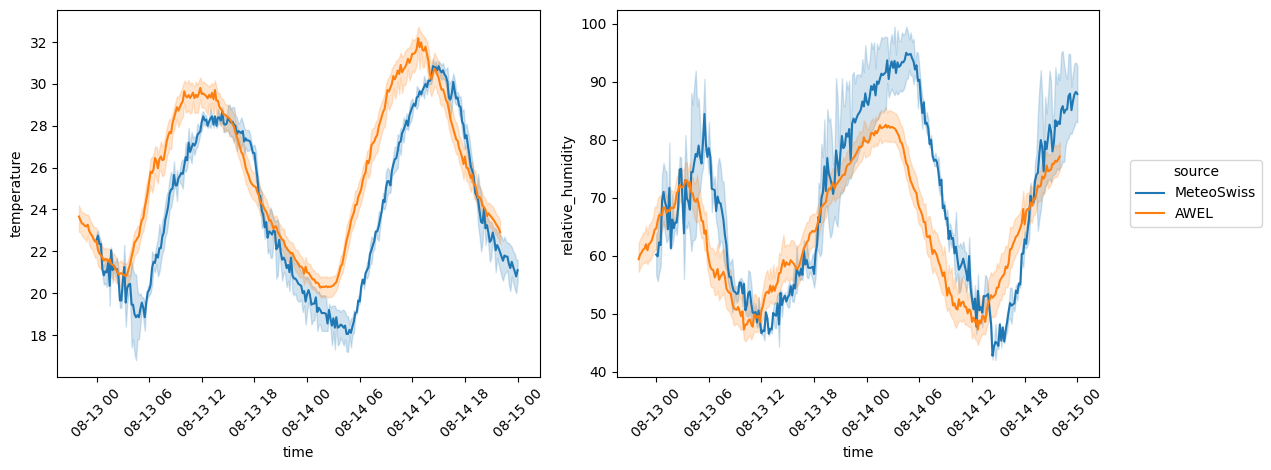
Then, given a list of climate variables and time period of interest, assemble the observations from the above sources into a single data frame:

variables = ["temperature", "relative_humidity"]
start = "08-13-2021"
end = "08-15-2021"

# from now on compare MeteoSwiss and AWEL data only
ts_client_dict = {
    "MeteoSwiss": meteoswiss_client,
    "AWEL": awel_client,
}

ts_df = pd.concat(
    [
        ts_client_dict[client_label]
        .get_ts_df(variables, start, end)
        .assign(source=client_label)
        for client_label in ts_client_dict
    ]
)
_ = plot_ts_by_source(ts_df, variables)

Why this matters? an example on computing urban climate indices

Nowadays the computation of climate indices often relies on global gridded products such as ERA5 reanalysis. However, these datasets can have major limitations, especially regarding the smoothing of local weather weather extremes due to interpolation (both spatial and temporal) (Wagner, 2025). These issues are exacerbated by the major spatial gaps in the underlying climate observation networks in developing regions such as Africa (van de Giesen et al., 2014, Vancutsem et al., 2010, World Meteorological Organization, 2020). Similarly, the observation networks in urban areas are too spatially sparse to accurately capture urban climate phenomena (Muller et al., 2013, Baklanov et al., 2018). Accordingly, reanalysis datasets have a rather coarse spatial resolution (e.g. 31 km for ERA5) which is likely too coarse given the spatial heterogeneity of cities and their impact on local climatic conditions.

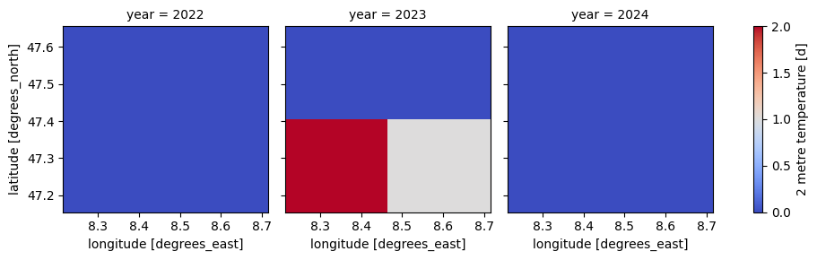
To overcome this, Meteora allows to easily retrieve data from multiple meteorological stations networks, which can then be used to compute climate indices at a higher spatial resolution. We will illustrate this by computing the number of tropical nights (i.e. nights where the minimum temperature remains above 20 °C) for June, July and August (JJA) for the years 2022 to 2024 using both ERA5 reanalysis data (downloaded with the “A01 - ERA5 data download” notebook) as well as local meteorological stations data from MeteoSwiss and AWEL:

# input data (temporal range)
start_year = 2022
end_year = 2024
start_month = 6
end_month = 8
# tropical night parameters
thresh = "20.0 degC"
freq = "YS"

# read ERA5 for the study region
era5_ds = xr.open_dataset(era5_filepath)

# compute tropical nights with xclim
era5_tn = xci.tn_days_above(
    era5_ds.resample(time="D").min()["t2m"], thresh=thresh, freq=freq
).rename("N. tropical nights")
era5_tn = era5_tn.assign_coords(year=era5_tn["time"].dt.year).swap_dims(
    {"time": "year"}
)
# plot the results
era5_tn.plot(
    col="year",
    cmap=cmap,
)

<xarray.plot.facetgrid.FacetGrid at 0x72d68438d550>

We will now use Meteora to retrieve temperature data from MeteoSwiss and AWEL stations for the same period and compute tropical nights from these observations:

tn_dfs = []
for label, client in ts_client_dict.items():
    ts_df = get_seasonal_ts_df(
        client,
        start_year,
        end_year,
        start_month,
        end_month,
        "temperature",
    )
    tn_df = (
        climate_indices.tn_days_above(
            ts_df,
            thresh=thresh,
            freq=freq,
        )
        .stack()
        .rename("tn")
        .reset_index()
        .assign(source=label)
    )
    # set geometry
    tn_df["geometry"] = tn_df["station_id"].map(
        client.stations_gdf["geometry"].to_crs(crs)
    )
    # set time as year only
    tn_df["time"] = tn_df["time"].dt.year
    # append it to the list
    tn_dfs.append(tn_df)
# put it together as a geo-data frame
tn_gdf = gpd.GeoDataFrame(pd.concat(tn_dfs, ignore_index=True))

# get global min/max values
vmin = tn_gdf["tn"].min()
vmax = tn_gdf["tn"].max()

plot_tn_facetgrid(tn_gdf, vmin=vmin, vmax=vmax, cmap=cmap, edgecolor="k")

---------------------------------------------------------------------------
TypeError                                 Traceback (most recent call last)
Cell In[10], line 12
      2 for label, client in ts_client_dict.items():
      3     ts_df = get_seasonal_ts_df(
      4         client,
      5         start_year,
   (...)      9         "temperature",
     10     )
     11     tn_df = (
---> 12         climate_indices.tn_days_above(
     13             ts_df,
     14             thresh=thresh,
     15             freq=freq,
     16         )
     17         .stack()
     18         .rename("tn")
     19         .reset_index()
     20         .assign(source=label)
     21     )
     22     # set geometry
     23     tn_df["geometry"] = tn_df["station_id"].map(
     24         client.stations_gdf["geometry"].to_crs(crs)
     25     )

File ~/checkouts/readthedocs.org/user_builds/meteora/checkouts/stable/meteora/climate_indices.py:1310, in tn_days_above(ts_df, thresh, freq, op, temperature_col, temperature_unit)
   1301 ts_da = _to_xarray_resampled(
   1302     ts_df,
   1303     temperature_col,
   (...)   1306     agg="min",
   1307 )
   1309 # compute index, transpose to have time as index and station ids as columns
-> 1310 return _to_pandas(xci.tn_days_above(ts_da, thresh=thresh, freq=freq, op=op))

File <boltons.funcutils.FunctionBuilder-82>:2, in tn_days_above(tasmin, thresh, freq, op)

File ~/checkouts/readthedocs.org/user_builds/meteora/checkouts/stable/.pixi/envs/doc/lib/python3.13/site-packages/xclim/core/units.py:1487, in declare_units.<locals>.dec.<locals>.wrapper(*args, **kwargs)
   1484 for name, dim in units_by_name.items():
   1485     check_units(bound_args.arguments.get(name), dim)
-> 1487 out = func(*args, **kwargs)
   1489 _check_output_has_units(out)
   1491 return out

File ~/checkouts/readthedocs.org/user_builds/meteora/checkouts/stable/.pixi/envs/doc/lib/python3.13/site-packages/xclim/indices/_threshold.py:2469, in tn_days_above(tasmin, thresh, freq, op)
   2467 thresh = convert_units_to(thresh, tasmin)
   2468 f = threshold_count(tasmin, op, thresh, freq, constrain=(">", ">="))
-> 2469 return to_agg_units(f, tasmin, "count", deffreq="D")

File ~/checkouts/readthedocs.org/user_builds/meteora/checkouts/stable/.pixi/envs/doc/lib/python3.13/site-packages/xclim/core/units.py:704, in to_agg_units(out, orig, op, dim, deffreq)
    701     out.attrs.update(units="1", is_dayofyear=np.int32(1), calendar=get_calendar(orig))
    703 elif op in ["count", "integral"]:
--> 704     m, freq_u_raw = infer_sampling_units(orig, deffreq=deffreq, dim=dim)
    705     orig_u = units2pint(orig)
    706     freq_u = str2pint(freq_u_raw)

File ~/checkouts/readthedocs.org/user_builds/meteora/checkouts/stable/.pixi/envs/doc/lib/python3.13/site-packages/xclim/core/units.py:532, in infer_sampling_units(da, deffreq, dim)
    507 """
    508 Infer a multiplier and the units corresponding to one sampling period.
    509 
   (...)    529     If the frequency has no corresponding units.
    530 """
    531 da = da[dim]
--> 532 freq = xr.infer_freq(da)
    533 if freq is None:
    534     if deffreq is None:

File ~/checkouts/readthedocs.org/user_builds/meteora/checkouts/stable/.pixi/envs/doc/lib/python3.13/site-packages/xarray/coding/frequencies.py:89, in infer_freq(index)
     87 if index.ndim != 1:
     88     raise ValueError("'index' must be 1D")
---> 89 elif not _contains_datetime_like_objects(Variable("dim", index)):
     90     raise ValueError("'index' must contain datetime-like objects")
     91 dtype = np.asarray(index).dtype

File ~/checkouts/readthedocs.org/user_builds/meteora/checkouts/stable/.pixi/envs/doc/lib/python3.13/site-packages/xarray/core/common.py:2102, in _contains_datetime_like_objects(var)
   2098 def _contains_datetime_like_objects(var: T_Variable) -> bool:
   2099     """Check if a variable contains datetime like objects (either
   2100     np.datetime64, np.timedelta64, or cftime.datetime)
   2101     """
-> 2102     return is_np_datetime_like(var.dtype) or contains_cftime_datetimes(var)

File ~/checkouts/readthedocs.org/user_builds/meteora/checkouts/stable/.pixi/envs/doc/lib/python3.13/site-packages/xarray/core/common.py:2070, in is_np_datetime_like(dtype)
   2068 def is_np_datetime_like(dtype: DTypeLike | None) -> bool:
   2069     """Check if a dtype is a subclass of the numpy datetime types"""
-> 2070     return np.issubdtype(dtype, np.datetime64) or np.issubdtype(dtype, np.timedelta64)

File ~/checkouts/readthedocs.org/user_builds/meteora/checkouts/stable/.pixi/envs/doc/lib/python3.13/site-packages/numpy/_core/numerictypes.py:534, in issubdtype(arg1, arg2)
    477 r"""
    478 Returns True if first argument is a typecode lower/equal in type hierarchy.
    479 
   (...)    531 
    532 """
    533 if not issubclass_(arg1, generic):
--> 534     arg1 = dtype(arg1).type
    535 if not issubclass_(arg2, generic):
    536     arg2 = dtype(arg2).type

TypeError: Cannot interpret 'datetime64[us, UTC]' as a data type

(C) OpenStreetMap contributors, Tiles style by Humanitarian OpenStreetMap Team hosted by OpenStreetMap France

In order to better appreciate the difference, we will plot the ERA5-based number of tropical nights using the same color scale as above:

# note that vmin and vmax come from the cell above in order to use the same color scale
grid = era5_tn.plot(
    col="year",
    cmap=cmap,
    vmin=vmin,
    vmax=vmax,
    add_colorbar=False,
)

cbar = grid.fig.colorbar(grid._mappables[0], ax=grid.axs.ravel().tolist())
cbar.set_label("N. tropical nights")

This shows how ERA5 underestimates the number of tropical nights compared to local meteorological stations and highlights the added value of using local meteorological stations data to compute urban climate indices.

References

[1]

A. Baklanov, C. S. B. Grimmond, D. Carlson, D. Terblanche, X. Tang, V. Bouchet, and A. Hovsepyan. From urban meteorology, climate and environment research to integrated city services. Urban Climate, 23:330–341, 2018.

[2]

C. Muller, L. Chapman, C. S. B. Grimmond, D. Young, and X. Cai. Sensors and the city: a review of urban meteorological networks. International Journal of Climatology, 33(7):1585–1600, 2013.

[3]

N. van de Giesen, R. Hut, and J. Selker. The trans-african hydro-meteorological observatory (tahmo). Wiley Interdisciplinary Reviews: Water, 1(4):341–348, 2014.

[4]

C. Vancutsem, P. Ceccato, T. Dinku, and S. J. Connor. Evaluation of modis land surface temperature data to estimate air temperature in different ecosystems over africa. Remote Sensing of Environment, 114(2):449–465, 2010.

[5]

Leonie Wagner. Rethinking weather model benchmarking: why stations matter more than grids. Jua blog, March 2025. URL: https://jua.ai/company/blog/stationbench-release (visited on 2026-03-06).

[6]

World Meteorological Organization. The gaps in the global basic observing network (gbon). Technical Report WMO-No. 1236, World Meteorological Organization, 2020.