Citizen weather stations quality checks

Citizen weather stations (CWS) provide an unprecedented potential for high-resolution climate modeling, especially in urban environments where the spatial density of stations can be very high (Meier et al., 2017, Muller et al., 2015). To that end, Meteora features the NetatmoClient, which makes it easy to access public data from Netatmo weather stations (one of the major CWS providers).

Like other low-cost sensors, Netatmo stations can be subject to radiative errors (Ahmed and Jänicke, 2025, Meier et al., 2017). Beyond such measurement biases, CWS are also prone to station-placement issues: many Netatmo stations report an identical geolocation - likely because an inadequate set up led to an automated location assignment based on the IP address of the wireless network (Meier et al., 2017) - while others are inadvertently set up indoors (Napoly et al., 2018).

Because of these issues, and since there is no guarantee that the scientific guidelines to properly set up meteorological stations have been met for CWS, performing a quality control (QC) of the collected CWS data is a crucial prerequisite before any analysis can be conducted. To that end, Meteora features the qc module, which is based on Napoly et al., (2018) (Napoly et al., 2018) and implements a set of statistically-based QC methods that control for common errors in CWS observations. Note that these QC methods are designed to detect stations with suspicious temperature measurements and therefore may not be appropriate to use on other meteorological variables.

import os

import contextily as cx
import geopandas as gpd
import matplotlib.pyplot as plt
import pandas as pd
import seaborn as sns

from meteora import clients, qc, settings, utils

figwidth = plt.rcParams["figure.figsize"][0]
figheight = plt.rcParams["figure.figsize"][1]

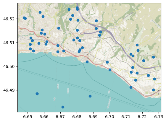
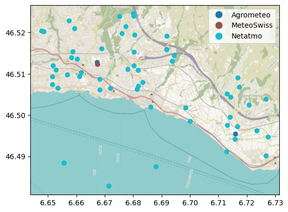
We will start by using the NetatmoClient to get CWS data for a bounding box in the Lavaux region of Switzerland. In order to use the NetatmoClient, we need to obtain a client ID and secret (see the detailed steps in the dedicated section of the Meteora documentation).

region = [6.6469, 46.4799, 6.7346, 46.5250]
crs = "epsg:4326"
client_id = os.getenv("NETATMO_CLIENT_ID", default="")
client_secret = os.getenv("NETATMO_CLIENT_SECRET", default="")
scale = "1hour"  # default is "30min"

# fallback to local files (to run notebooks programatically without interactive auth
netatmo_ts_filepath = "data/lavaux-netatmo-ts-df.csv"
netatmo_stations_filepath = "data/lavaux-netatmo-cws.gpkg"
use_netatmo_files = not client_id or not client_secret

Given the client ID and secret, we can pass them to the instantiation of the NetatmoClient, which will then open a browser window asking us to authorize our application (that we used to get the client ID and secret) to access the data from the Netatmo weather stations. After accepting, we will be redirected to the page with the list of your accounts applications. At the end of the URL bar there will be an authorization code preceded by code=, which we will have to copy and enter into the input window that will appear when we execute the cell below:

if not use_netatmo_files:
    # query Netatmo data from the API
    client = clients.NetatmoClient(region, client_id, client_secret)
    stations_gdf = client.stations_gdf
else:
    # fallback to a local file when interactive auth is not possible
    stations_gdf = gpd.read_file(netatmo_stations_filepath)
    if settings.STATIONS_ID_COL in stations_gdf.columns:
        stations_gdf = stations_gdf.set_index(settings.STATIONS_ID_COL)
    client = None

Like in any other Meteora client, we can start by plotting the station locations:

ax = stations_gdf.plot()
cx.add_basemap(ax=ax, crs=stations_gdf.crs, attribution="")

(C) OpenStreetMap contributors, Tiles style by Humanitarian OpenStreetMap Team hosted by OpenStreetMap France

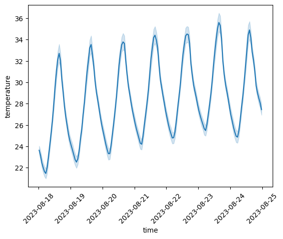
Let us now get a time series of data during a heatwave in August 2023, defined as at least 3 consecutive days with an average temperature over 25$^{\circ}$C (based on the heat level warning definitions by MeteoSwiss):

variables = ["temperature"]
start = "18-08-2023"
end = "25-08-2023"

if use_netatmo_files:
    # fallback to a local file when interactive auth is not possible
    long_ts_df = pd.read_csv(
        netatmo_ts_filepath,
        index_col=[settings.STATIONS_ID_COL, settings.TIME_COL],
        parse_dates=True,
    )
    long_ts_df = long_ts_df[variables]
else:
    # query Netatmo data from the API
    long_ts_df = client.get_ts_df(variables, start, end, scale=scale)

/tmp/ipykernel_1300/126283522.py:7: UserWarning: Could not infer format, so each element will be parsed individually, falling back to `dateutil`. To ensure parsing is consistent and as-expected, please specify a format.
  long_ts_df = pd.read_csv(

The get_ts_df method of all Meteora clients returns a long-form time series data frame, multi-indexed by stations (first level) and time (second level) and with variables as columns. However, the qc module expects a wide-form time series data frame instead, where each cell represents the temperature measurement at a given time (index) and station (columns). See the “Data structures” section of the Meteora documentation for more details. We can use the meteora.utils.long_to_wide function to convert it:

ts_df = utils.long_to_wide(long_ts_df)

Since there are several dozen CWS in the study area, we can use the seaborn.lineplot function to plot the mean and 95% confidence interval at each temporal cross-section:

ax = sns.lineplot(long_ts_df.reset_index(), x="time", y="temperature")
ax.tick_params(axis="x", labelrotation=45)

Quality control pipeline

Rather than applying each quality check by hand, Meteora bundles them into meteora.qc.QCPipeline, which in line with the approach of scikit-learn pipelines, chains an ordered sequence of QC steps and applies them to a (wide) time series data frame.

Based on the literature meier2017crowdsourcing,napoly2018qc will:

1. flag mislocated stations, likely due to an incorrect set up that led to automatic location assignment based on the IP address of the wireless network;

2. flag unreliable stations, with a high proportion (customizable) of non-valid measurements;

3. adjust temperature measurements based on station elevation to account for the atmospheric lapse rate;

4. flag outlier stations, which show a high proportion of measurements that largely deviate from a normal distribution (especially in the upper tail due to radiative errors);

5. flag indoor stations, whose measurements show low correlation with the spatial median.

See the section “The individual QC steps” for more details on each QC step. Let us now apply this to our data:

elevation_col = "altitude"  # required to enable elevation adjustment
pipeline = qc.QCPipeline(
    stations=stations_gdf,
    elevation=elevation_col,
)
qc_ts_df = pipeline.apply(ts_df)
print(f"{ts_df.shape[1]} stations before QC, {qc_ts_df.shape[1]} after")
pipeline.discarded_

51 stations before QC, 38 after

{'flag_mislocated': ['70:ee:50:00:18:ca',
  '70:ee:50:3f:77:f0',
  '70:ee:50:5f:19:16'],
 'flag_unreliable': ['70:ee:50:27:41:ac', '70:ee:50:90:79:f4'],
 'adjust_elevation': [],
 'flag_outliers': ['70:ee:50:00:eb:2a', '70:ee:50:28:89:d4'],
 'flag_indoor': ['70:ee:50:00:71:0a',
  '70:ee:50:00:78:82',
  '70:ee:50:27:66:ba',
  '70:ee:50:29:2c:ca',
  '70:ee:50:65:70:a2',
  '70:ee:50:9c:e8:d6']}

Calling apply returns the quality-controlled data frame (with the flagged stations dropped) and records the stations discarded by each step in the discarded_ attribute (keyed by the step/function name).

The individual QC steps

The pipeline above ran the default sequence of steps - meteora.settings.DEFAULT_QC_STEPS - which we now go through one by one. For each step we explain what it does, which parameter (and meteora.settings default) controls it, and use the stations it flagged - readily available in pipeline.discarded_ - to visualize its effect. Note that each built-in step is also exposed as a standalone function in the qc module, should one prefer to run it on its own.

Several of the steps below are illustrated by comparing the time series of the discarded and kept stations. Let us first define a small comparison_lineplot helper:

def comparison_lineplot(
    ts_df,
    discard_stations,
    *,
    label_discarded="discarded",
    label_kept="kept",
    individual_discard_lines=False,
    ax=None,
):
    """Plot the time series of the discarded and kept stations separately."""
    data = pd.concat(
        [
            _ts_df.reset_index()
            .melt(value_name="temperature", id_vars="time")
            .assign(label=label)
            for _ts_df, label in zip(
                [
                    ts_df[discard_stations],
                    ts_df.drop(columns=discard_stations, errors="ignore"),
                ],
                [label_discarded, label_kept],
            )
        ],
        ignore_index=True,
    )
    if ax is None:
        _, ax = plt.subplots()
    if individual_discard_lines:
        # avoid warnings about matplotlib converters
        pd.plotting.register_matplotlib_converters()
        sns.lineplot(
            data[data["label"] == label_kept],
            x="time",
            y="temperature",
            hue="label",
            ax=ax,
        )
        data[data["label"] == label_discarded].set_index("time").rename(
            columns={"temperature": label_discarded}
        ).plot(ax=ax)
    else:
        sns.lineplot(data, x="time", y="temperature", hue="label", ax=ax)
        ax.tick_params(axis="x", labelrotation=45)
    return ax

Mislocated stations

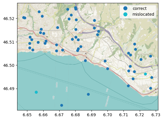
The first step, "flag_mislocated", filters stations purely from their geolocation, flagging those that share an identical location. As noted by Meier et al. (2017) (Meier et al., 2017), many Netatmo stations show identical geolocation, which is likely because an inadequate set up “led to automated location assignment based on the IP address of the wireless network” (Napoly et al., 2018) (page 4). This step takes no parameters (it is purely geometric) and is skipped when no stations are provided. Let us plot the flagged stations on a map:

mislocated_stations = pipeline.discarded_["flag_mislocated"]
ax = stations_gdf.assign(
    label=[
        "mislocated" if i in mislocated_stations else "correct"
        for i in stations_gdf.index
    ]
).plot("label", legend=True)
cx.add_basemap(ax, crs=stations_gdf.crs, attribution="")

(C) OpenStreetMap contributors, Tiles style by Humanitarian OpenStreetMap Team hosted by OpenStreetMap France

As we can see, some of the mislocated stations, but not all of them, are on Lake Geneva. The other stations on the lake are likely mislocated too and can be filtered out using an ad-hoc method.

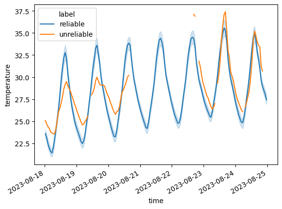
Unreliable stations

The "flag_unreliable" step filters out stations with too few valid observations during the study period. The maximum proportion of missing observations is set by the unreliable_threshold keyword argument (defaulting to meteora.settings.UNRELIABLE_THRESHOLD). Since there are only a few such stations, we use individual_discard_lines=True so that each is drawn as its own line (rather than a mean plus confidence interval), which lets us appreciate the periods with non-valid data:

comparison_lineplot(
    ts_df,
    pipeline.discarded_["flag_unreliable"],
    label_discarded="unreliable",
    label_kept="reliable",
    individual_discard_lines=True,
)

<Axes: xlabel='time', ylabel='temperature'>

Elevation adjustment

Due to the atmospheric lapse rate, stations at lower elevations are usually expected to be consistently warmer than their counterparts at higher elevations (except under, e.g., the occurrence of inversion). The "adjust_elevation" step therefore adjusts the time series rather than discarding stations - otherwise we may find, e.g., that a given station is consistently warmer because of an incorrect set up when in reality the difference is due to the elevation. The adjustment uses the per-station elevation passed to the step (station_elevation_ser) and the atmospheric_lapse_rate keyword argument (defaulting to meteora.settings.ATMOSPHERIC_LAPSE_RATE). Being a transform, this step discards no stations (its entry in discarded_ is empty); to illustrate its effect we can apply meteora.qc.adjust_elevation directly and map the difference between the average adjusted and unadjusted temperature at each station:

adj_ts_df, _ = qc.adjust_elevation(
    ts_df,
    station_elevation_ser=stations_gdf["altitude"],
)
ax = stations_gdf.assign(diff=adj_ts_df.mean() - ts_df.mean()).plot(
    "diff",
    legend=True,
    legend_kwds={
        "label": "$\\overline{T_{adj}} - \\overline{T} \\quad [\\circ C]$",
        "shrink": 0.6,
    },
)
cx.add_basemap(ax, crs=stations_gdf.crs, attribution="")
stations_gdf["altitude"].describe()[["mean", "min", "max"]]

mean    504.745763
min     370.000000
max     764.000000
Name: altitude, dtype: float64

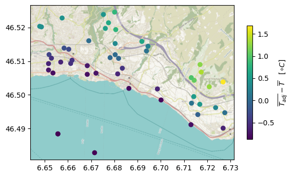
(C) OpenStreetMap contributors, Tiles style by Humanitarian OpenStreetMap Team hosted by OpenStreetMap France

Stations at higher elevations are added about 1.5 $^{\circ}$C whereas the ones at lower elevations are subtracted less than that (because of the smaller elevation difference between the mean and the minimum than between the maximum and the mean).

Outlier stations

The "flag_outliers" step detects stations whose measurements show suspicious deviations from a normal distribution (based on a modified z-score using a robust Qn variance estimator). It accepts the low_alpha and high_alpha keyword arguments - the lower- and upper-tail significance levels that lead to flagging a measurement as an outlier (defaulting to meteora.settings.OUTLIER_LOW_ALPHA and meteora.settings.OUTLIER_HIGH_ALPHA) - and station_outlier_threshold, the maximum proportion of outlier measurements after which the station is flagged (defaulting to meteora.settings.STATION_OUTLIER_THRESHOLD). As noted by Meier et al. (2017) (Meier et al., 2017), one of the main issues with Netatmo data are stations located in non-shaded areas, resulting in radiative errors, which is why the upper-tail threshold is by default less permissive than its lower-tail counterpart:

comparison_lineplot(
    ts_df,
    pipeline.discarded_["flag_outliers"],
    label_discarded="outlier",
    label_kept="non-outlier",
)

<Axes: xlabel='time', ylabel='temperature'>

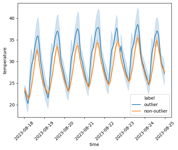
Stations labeled as outliers clearly display an amplified temperature variation, especially for the maximum temperatures - in line with the radiative errors suggested by Meier et al. (2017) (Meier et al., 2017).

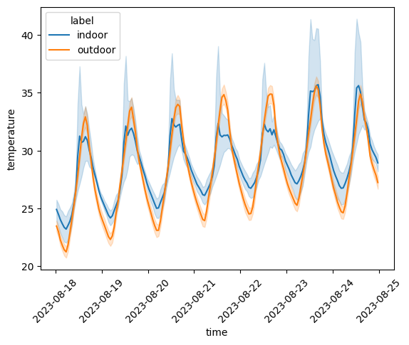
Indoor stations

Netatmo stations may also be set indoors, in which case their diurnal cycles are assumed to be less correlated with the one from outdoor stations (Napoly et al., 2018). The "flag_indoor" step flags stations whose Pearson correlation with the overall station median is below the station_indoor_corr_threshold keyword argument (defaulting to meteora.settings.STATION_INDOOR_CORR_THRESHOLD). We can plot the time series of temperature measurements for indoor and outdoor stations separately:

comparison_lineplot(
    ts_df,
    pipeline.discarded_["flag_indoor"],
    label_discarded="indoor",
    label_kept="outdoor",
)

<Axes: xlabel='time', ylabel='temperature'>

Customizing the pipeline

The default pipeline can be customized in several ways: running it without the station metadata (skipping the steps that need it), tuning each step’s parameters through step_kwargs, inserting transforming steps that modify the measurements instead of discarding stations (e.g. mask_outliers), adding built-in steps that are not part of the default sequence (e.g. the spatial buddy check), and even plugging in our own callables. The following sections cover each of these in turn. In every case a step is given either as the name of a built-in meteora.qc function or as any callable matching the signature step(ts_df, **kwargs) -> (ts_df, discarded_station_ids).

Running without station metadata

The pipeline does not require the station locations or elevation: when they are not provided, the steps that need them are simply skipped. Running the default pipeline with no arguments therefore omits the mislocated-station flagging and the elevation adjustment:

pipeline = qc.QCPipeline()
qc_ts_df = pipeline.apply(ts_df)
print(f"{ts_df.shape[1]} stations before QC, {qc_ts_df.shape[1]} after")
pipeline.discarded_

51 stations before QC, 39 after

{'flag_unreliable': ['70:ee:50:27:41:ac', '70:ee:50:90:79:f4'],
 'flag_outliers': ['70:ee:50:00:eb:2a',
  '70:ee:50:5e:f6:ec',
  '70:ee:50:5f:19:16'],
 'flag_indoor': ['70:ee:50:00:71:0a',
  '70:ee:50:00:78:82',
  '70:ee:50:27:66:ba',
  '70:ee:50:28:89:d4',
  '70:ee:50:29:2c:ca',
  '70:ee:50:65:70:a2',
  '70:ee:50:9c:e8:d6']}

Tuning step parameters

Each step’s parameters are supplied through the step_kwargs list, one dict per step and positionally matched to steps. Any step whose entry is omitted - by not passing step_kwargs at all - or left empty ({}) falls back to the parameter defaults defined in meteora.settings.

unreliable_threshold = 0.2
atmospheric_lapse_rate = 0.0065  # in C / m
low_alpha = 0.01
high_alpha = 0.95
station_outlier_threshold = 0.2
station_indoor_corr_threshold = 0.9

# each step receives its own keyword-argument dict, positionally matched to `steps`;
# the per-station elevation series is passed to the `adjust_elevation` step
default_step_kwargs = [
    {},  # flag_mislocated (purely geometric)
    {"unreliable_threshold": unreliable_threshold},
    {
        "atmospheric_lapse_rate": atmospheric_lapse_rate,
    },
    {
        "low_alpha": low_alpha,
        "high_alpha": high_alpha,
        "station_outlier_threshold": station_outlier_threshold,
    },
    {"station_indoor_corr_threshold": station_indoor_corr_threshold},
]
pipeline = qc.QCPipeline(
    stations=stations_gdf,
    elevation="altitude",
    steps=settings.DEFAULT_QC_STEPS,
    step_kwargs=default_step_kwargs,
)
_ = pipeline.apply(ts_df)
pipeline.discarded_

{'flag_mislocated': ['70:ee:50:00:18:ca',
  '70:ee:50:3f:77:f0',
  '70:ee:50:5f:19:16'],
 'flag_unreliable': ['70:ee:50:27:41:ac', '70:ee:50:90:79:f4'],
 'adjust_elevation': [],
 'flag_outliers': ['70:ee:50:00:eb:2a', '70:ee:50:28:89:d4'],
 'flag_indoor': ['70:ee:50:00:71:0a',
  '70:ee:50:00:78:82',
  '70:ee:50:27:66:ba',
  '70:ee:50:29:2c:ca',
  '70:ee:50:65:70:a2',
  '70:ee:50:9c:e8:d6']}

Flagging vs. transforming steps

There are two main types of QC steps depending on how apply handles their output:

• Flagging steps discard whole stations: they return the list of suspicious station ids - recorded in discarded_ - and leave the measurements untouched. All the flag_* steps (flag_mislocated, flag_unreliable, flag_outliers, flag_indoor, flag_buddies) are of this kind.

• Transforming steps instead modify the measurements and discard no station (their discarded_ entry is always empty). adjust_elevation is one: it shifts each station’s temperature by the lapse-rate correction rather than flagging anyone - which is why, although it belongs to the default sequence, it never contributes any discarded station.

A second transforming step, deliberately left out of meteora.settings.DEFAULT_QC_STEPS, is meteora.qc.mask_outliers. It reuses the exact same robust (median/Qn) z-score as flag_outliers, but instead of discarding entire stations it replaces the individual outlier measurements with NaN - closer to the m2 level of CrowdQC+ (Fenner et al., 2021), which flags values rather than whole stations. Being a transform, it returns the modified data frame and an empty discard list, and can be applied on its own or inserted anywhere in a pipeline:

masked_ts_df, discarded = qc.mask_outliers(ts_df)
n_masked = int(masked_ts_df.isna().sum().sum() - ts_df.isna().sum().sum())
print(f"{n_masked} measurements masked as outliers; stations discarded: {discarded}")

116 measurements masked as outliers; stations discarded: []

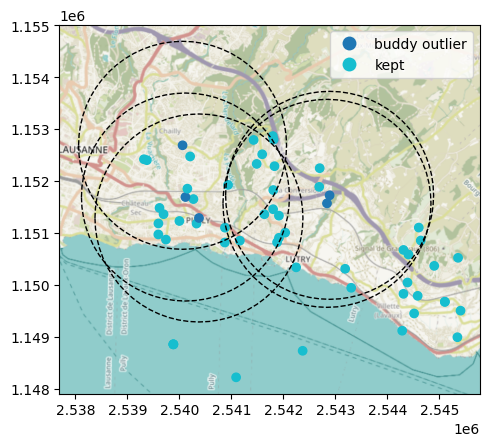
Spatial buddy check

The flag_outlier step compares each station against the whole network. We can complement it with a spatial buddy check, which instead compares each station only against its neighbours (its “buddies”) within a given radius (B\aaserud et al., 2020, Fenner et al., 2021). In meteora, this is implemented as the flag_buddies step, which is deliberately not part of meteora.settings.DEFAULT_QC_STEPS but is easy to add through the steps argument. Its neighbourhood is set by buddy_radius (in meters, defaulting to meteora.settings.BUDDY_RADIUS) and buddy_min_n (the minimum number of buddies required to evaluate a station, defaulting to meteora.settings.BUDDY_MIN_N); it reuses the outlier statistics (low_alpha, high_alpha, station_outlier_threshold, defaulting to the meteora.settings.BUDDY_* values) in its own step_kwargs dict. Let us add it to the default sequence and compare:

buddy_radius = 2000  # in meters
pipeline_buddy = qc.QCPipeline(
    stations=stations_gdf,
    steps=[*settings.DEFAULT_QC_STEPS, "flag_buddies"],
    step_kwargs=[*default_step_kwargs, {"buddy_radius": buddy_radius}],
)
qc_buddy_ts_df = pipeline_buddy.apply(ts_df)
print(
    f"{qc_ts_df.shape[1]} stations kept without the buddy check, "
    f"{qc_buddy_ts_df.shape[1]} with it"
)
pipeline_buddy.discarded_["flag_buddies"]

39 stations kept without the buddy check, 32 with it

['70:ee:50:03:0d:44',
 '70:ee:50:33:2f:60',
 '70:ee:50:3f:65:14',
 '70:ee:50:5f:39:a4',
 '70:ee:50:80:0e:0e']

The buddy check flags the additional stations above. Since it is a spatial check, we visualize its effect on a map: each flagged station is shown together with a dashed circle delimiting the buddy_radius neighbourhood it was compared against (note that some flagged stations may already have been caught by the earlier steps):

buddy_flagged = pipeline_buddy.discarded_["flag_buddies"]
# project to LV95 so that `buddy_radius` (in meters) maps to true distances
stations_lv95_gdf = stations_gdf.to_crs("epsg:2056")
ax = stations_lv95_gdf.assign(
    label=[
        "buddy outlier" if i in buddy_flagged else "kept"
        for i in stations_lv95_gdf.index
    ]
).plot("label", legend=True)
# dashed circle delimiting each flagged station's `buddy_radius` neighbourhood
stations_lv95_gdf.loc[buddy_flagged].buffer(buddy_radius).boundary.plot(
    ax=ax, color="black", linestyle="--", linewidth=1
)
cx.add_basemap(ax, crs=stations_lv95_gdf.crs, attribution="")

Custom steps

Each step can be given either as a string naming a built-in function of meteora.qc (as in the sequences above), or directly as any callable with the signature step(ts_df, **kwargs) -> (ts_df, discarded_station_ids): station-discarding steps return ts_df unchanged together with the ids to drop, while transforms (e.g. the elevation adjustment) return a new ts_df and an empty list. We can therefore freely interleave built-in names and our own functions in the steps list, supplying each step’s parameters through the positionally-matched step_kwargs list. As an example, the callable below flags systematically sunlit stations - those that overheat at the same hour every day, a recurring radiative bias that the per-measurement flag_outliers step can miss because it is too small a fraction of the record. It is a deliberately simplified version of the method of Bosch et al. (in prep.) (Climatology Group of the University of Bern, 2026), dropped into the pipeline right after the flag_outliers step:

def sunlit_stations(ts_df, *, contrast_threshold=1.5):
    """Flag systematically sunlit stations: a recurring, time-locked warm peak.

    Robust cross-station z-score (median centre, MAD scale), then for each station the
    median-over-days hour-of-day profile; a station is flagged when its warmest hour
    exceeds its own baseline (the median across hours) by more than
    ``contrast_threshold``. Simplified from Bosch et al. (in prep.), whose full method
    adds a permutation significance test with false-discovery-rate control.
    """
    centered = ts_df.sub(ts_df.median(axis="columns"), axis="index")
    z = centered.div(1.4826 * centered.abs().median(axis="columns"), axis="index")
    profile = z.groupby(z.index.hour).median()  # hour-of-day median per station
    contrast = profile.max() - profile.median()  # peak vs the station's own baseline
    return ts_df, list(contrast.index[contrast > contrast_threshold])


custom_pipeline = qc.QCPipeline(
    stations=stations_gdf,
    steps=[
        "flag_mislocated",
        "flag_unreliable",
        "adjust_elevation",
        "flag_outliers",
        sunlit_stations,
        "flag_indoor",
    ],
)
_ = custom_pipeline.apply(ts_df)
custom_pipeline.discarded_

{'flag_mislocated': ['70:ee:50:00:18:ca',
  '70:ee:50:3f:77:f0',
  '70:ee:50:5f:19:16'],
 'flag_unreliable': ['70:ee:50:27:41:ac', '70:ee:50:90:79:f4'],
 'adjust_elevation': [],
 'flag_outliers': ['70:ee:50:00:eb:2a',
  '70:ee:50:28:89:d4',
  '70:ee:50:5e:f6:ec'],
 'sunlit_stations': ['70:ee:50:00:71:0a',
  '70:ee:50:00:ba:d6',
  '70:ee:50:03:0d:44',
  '70:ee:50:03:8a:d6',
  '70:ee:50:03:8b:f6',
  '70:ee:50:22:bd:30',
  '70:ee:50:28:af:26',
  '70:ee:50:3b:ed:d2',
  '70:ee:50:3f:65:14',
  '70:ee:50:5f:3c:62',
  '70:ee:50:6b:7a:56',
  '70:ee:50:73:f5:00',
  '70:ee:50:74:6f:d0',
  '70:ee:50:74:70:c2',
  '70:ee:50:80:05:46',
  '70:ee:50:80:0e:0e',
  '70:ee:50:90:70:e6',
  '70:ee:50:96:a9:22',
  '70:ee:50:9c:e8:d6'],
 'flag_indoor': ['70:ee:50:65:70:a2']}

Comparison with official data

Finally, we can compare the time series of temperature measurements of the CWS data (before and after QC) with its counterpart from official stations. To that end, we will get the data from Agrometeo and MeteoSwiss:

# official
# specify the crs for both clients (they default to other CRSs: epsg:21781 for
# Agrometeo, the Swiss LV95 epsg:2056 for MeteoSwiss), otherwise the lon/lat `region`
# bounding box is misinterpreted and no stations are matched
agrometeo_client = clients.AgrometeoClient(region, crs=crs)
meteoswiss_client = clients.MeteoSwissClient(region, crs=crs)

ax = pd.concat(
    [
        stations_gdf.assign(source=label).to_crs(crs)
        for label, stations_gdf in {
            "Netatmo": stations_gdf,
            "Agrometeo": agrometeo_client.stations_gdf,
            "MeteoSwiss": meteoswiss_client.stations_gdf,
        }.items()
    ]
).plot("source", legend=True)
cx.add_basemap(ax, crs=crs, attribution="")

There are only a few official stations in the study area compared with the high spatial density of Netatmo CWS. Let us now get the time series of temperature data for the study period:

# specify hourly `scale` for Agrometeo, otherwise is 10-minutes.
agrometeo_ts_df = agrometeo_client.get_ts_df(variables, start, end, scale="hour")
meteoswiss_ts_df = meteoswiss_client.get_ts_df(variables, start, end)

We can now plot the time series separately. To have more flexibility, we will use the long-form data frames (note that we thus need to exclude the discarded stations, which were dropped from the quality-controlled wide-form data frame but not from the long-form one):

all_discards = pipeline.discarded_stations
ax = sns.lineplot(
    pd.concat(
        [
            ts_df.assign(label=label)
            for ts_df, label in zip(
                [
                    long_ts_df.drop(all_discards, errors="ignore"),
                    long_ts_df[
                        long_ts_df.index.get_level_values("station_id").isin(
                            all_discards
                        )
                    ],
                    pd.concat([agrometeo_ts_df, meteoswiss_ts_df]),
                ],
                ["CWS (QC)", "CWS (Discarded)", "Official"],
            )
        ]
    )
    .droplevel("station_id")
    .reset_index(),
    x="time",
    y="temperature",
    hue="label",
)
ax.tick_params(axis="x", labelrotation=45)

/home/docs/checkouts/readthedocs.org/user_builds/meteora/checkouts/stable/.pixi/envs/doc/lib/python3.13/site-packages/matplotlib/dates.py:449: UserWarning: no explicit representation of timezones available for np.datetime64
  d = d.astype('datetime64[us]')

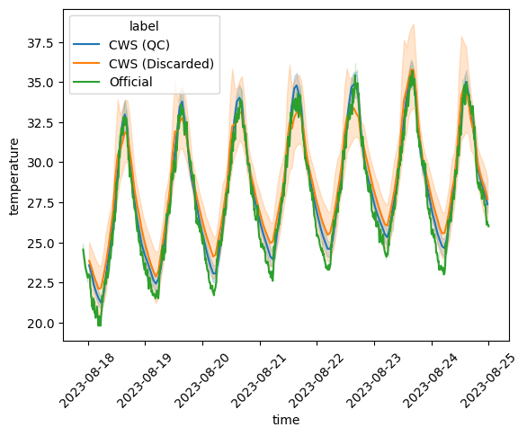
We can observe how, unlike the discarded CWS, the CWS that pass QC have a very similar trend as the official stations. Although this is beyond the scope of this notebook, note that even after QC, CWS seem to be slightly warmer than the official stations, but this may be due to elevation differences as well as the urban heat island effect.

References

[1]

Shakir Ahmed and Britta Jänicke. Comparison and assessment of air temperature observations using all-in-one and low-cost sensors in an urban environment. Transactions in Earth, Environment, and Sustainability, 3(1):28–50, 2025.

[2]

Line B\aaserud , Cristian Lussana, Thomas N. Nipen, Ivar A. Seierstad, Louise Oram, and Trygve Aspelien. TITAN automatic spatial quality control of meteorological in-situ observations. Advances in Science and Research, 17:153–163, 2020.

[3] (1,2)

Daniel Fenner, Benjamin Bechtel, Matthias Demuzere, Jonas Kittner, and Fred Meier. Outdoor air temperature observations from citizen weather stations: CrowdQC+, a quality-control package for citizen weather station data. Frontiers in Earth Science, 9:720747, 2021.

[4] (1,2,3,4,5,6)

Fred Meier, Daniel Fenner, Tom Grassmann, Marco Otto, and Dieter Scherer. Crowdsourcing air temperature from citizen weather stations for urban climate research. Urban Climate, 19:170–191, 2017.

[5]

C. L. Muller, L. Chapman, S. Johnston, C. Kidd, S. Illingworth, G. Foody, and R. R. Leigh. Crowdsourcing for climate and atmospheric sciences: current status and future potential. International Journal of Climatology, 35(11):3185–3203, 2015.

[6] (1,2,3,4)

Adrien Napoly, Tom Grassmann, Fred Meier, and Daniel Fenner. Development and application of a statistically-based quality control for crowdsourced air temperature data. Frontiers in Earth Science, pages 118, 2018.

[7]

Climatology Group of the University of Bern. Detecting systematically sunlit citizen weather stations to extend crowdsourced urban heat monitoring beyond the night. Manuscript in preparation, 2026.