Radiation bias correction for low-cost temperature sensors#

Low-cost temperature devices (LCD) are increasingly used to densify urban meteorological networks at low deployment cost (Muller et al., 2013, Wong et al., 2025). However, these devices often lack proper radiation shields, which causes their temperature readings to be systematically biased upward during daytime (Bell et al., 2015, Bosch and Burger, 2026, Büchau, 2018, Chapman et al., 2016, Cornes et al., 2020).

The meteora.bias_correction module provides tools to apply pre-trained correction models that remove this radiation-driven bias. Each model captures the radiation-to-temperature-bias relationship for a specific sensor type and can be shared as a scikit-learn pipeline serialized with skops on Hugging Face Hub.

This notebook shows the following pipeline:

Retrieve LCD temperature data from the AWEL network of Decentlab sensors in Zurich (Amt für Abfall, Wasser, Energie und Luft, 2026) using meteora.clients.AWELClient.
Retrieve reference automated weather station (AWS) air temperature and shortwave radiation data from the MeteoSwiss automated observation network (SwissMetNet) using meteora.clients.MeteoSwissClient.
Load a pre-trained correction model from Hugging Face Hub at martibosch/decentlab-bias-correction.
Apply the correction and compare the results.

The pre-trained model used here is fitted based on the temperature readings of a Decentlab sensor and the temperature and shortwave radiation measurements from a reference AWS from SwissMetNet at Zollikofen (Switzerland), collocated alongside further LCD models in an intercomparison field study in summer 2025 (Bosch and Burger, 2026).

Note

This notebook requires the sk and xvec optional extras as well as the interpret library for the pre-trained correction models. The requirements can be installed as in, e.g.:

pip install interpret meteora[sk,xvec]

import contextily as cx
import matplotlib.pyplot as plt
import pandas as pd
import seaborn as sns
from huggingface_hub import hf_hub_download
from sklearn.linear_model import LinearRegression
from sklearn.pipeline import Pipeline
from skops import io as skops_io

from meteora import clients, settings, utils
from meteora.bias_correction import (
    BestScaleRadiationTransformer,
    apply_bias_correction,
    load_correction_model,
    parse_hf_path,
)

figwidth, figheight = plt.rcParams["figure.figsize"]

region = "Zurich, Switzerland"
start = "2023-07-01"
end = "2023-07-31"

LCD sensor data#

We can start by getting LCD data for our study area, in this case, the city of Zurich (Switzerland). The AWEL (Amt für Abfall, Wasser, Energie und Luft) network operates Decentlab LoRa temperature sensors across the Zurich agglomeration. We use the AWELClient to retrieve temperature measurements for July 2023:

awel_client = clients.AWELClient(region)
lcd_ts_df = utils.long_to_wide(
    awel_client.get_ts_df(settings.ECV_TEMPERATURE, start=start, end=end)
)
lcd_stations_gdf = awel_client.stations_gdf
lcd_ts_df.head()

station_id	530	534	2651	2652	2653	2655	2656	2657	2659	2679	2680	2682	2683	2688	2689	2695	2696	2697	2810
time
2023-07-01 00:00:00+02:00	NaN	17.01	15.82	16.78	14.53	16.30	NaN	16.30	16.70	16.20	17.50	16.92	16.28	16.68	16.96	16.64	16.04	15.73	16.08
2023-07-01 00:10:00+02:00	16.75	17.14	15.87	16.82	14.54	16.41	NaN	NaN	16.75	16.17	17.52	16.95	16.27	16.78	17.14	16.61	16.03	15.60	16.05
2023-07-01 00:20:00+02:00	16.72	17.14	15.87	16.91	14.49	16.51	NaN	16.35	16.79	16.38	17.56	17.01	16.34	16.83	17.15	16.67	16.03	15.55	16.04
2023-07-01 00:30:00+02:00	16.72	17.25	15.90	17.07	14.49	16.57	NaN	16.43	16.86	16.57	17.54	17.16	16.28	16.95	17.26	16.71	16.09	15.44	15.97
2023-07-01 00:40:00+02:00	16.69	17.14	15.95	17.11	14.49	16.68	NaN	16.47	16.87	16.59	17.48	17.31	NaN	17.11	17.32	16.75	15.98	15.40	15.99

Reference weather station data#

The bias correction relies on co-located shortwave radiation measurements to predict the radiation-induced temperature offset. We use the MeteoSwissClient to fetch air temperature and global shortwave radiation from official MeteoSwiss automated weather stations in the same region:

aws_client = clients.MeteoSwissClient(region)
aws_ts_df = aws_client.get_ts_df(
    [settings.ECV_TEMPERATURE, settings.ECV_RADIATION_SHORTWAVE],
    start=start,
    end=end,
)
aws_ts_df.head()

		temperature	radiation_shortwave
station_id	time
REH	2023-07-01 00:00:00+00:00	15.6	0.0
	2023-07-01 00:10:00+00:00	15.7	0.0
	2023-07-01 00:20:00+00:00	15.5	0.0
	2023-07-01 00:30:00+00:00	15.5	0.0
	2023-07-01 00:40:00+00:00	15.5	1.0

We can visualise both station networks on a shared map:

colors = sns.color_palette()
fig, ax = plt.subplots()
aws_client.stations_gdf.to_crs(lcd_stations_gdf.crs).plot(
    ax=ax, color=colors[0], label="AWS (MeteoSwiss)"
)
lcd_stations_gdf.plot(ax=ax, color=colors[1], label="LCD (AWEL)")
ax.legend()
cx.add_basemap(ax, crs=lcd_stations_gdf.crs, attribution="")

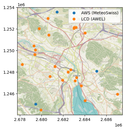
../_images/aa6711888c73798e98e538adb4583b29fc02a704da78e6d1080fcb0b1bb62e68.png

(C) OpenStreetMap contributors, Tiles style by Humanitarian OpenStreetMap Team hosted by OpenStreetMap France

For the spatial matching between LCD stations and their nearest AWS reference (needed to assign each LCD sensor the correct radiation time series), we can convert the long-form data frame and station geo-data frame to a vector data cube:

Applying bias correction#

We call apply_bias_correction, passing the HuggingFace Hub repository string directly as the model. Since the pipeline is serialized with skops, it is recommended to first inspect the non-sklearn types it contains as a security step before deserialization:

model_str = "martibosch/lcd-bias-correction/decentlab.skops"
repo_id, filename = parse_hf_path(model_str)

trusted = skops_io.get_untrusted_types(file=hf_hub_download(repo_id, filename))
print("Types to review before trusting:")
for t in trusted:
    print(f"  {t}")

Warning: You are sending unauthenticated requests to the HF Hub. Please set a HF_TOKEN to enable higher rate limits and faster downloads.

Types to review before trusting:
  interpret.glassbox._ebm._ebm.ExplainableBoostingRegressor
  meteora.bias_correction.BestScaleRadiationTransformer

After reviewing the listed types, we can pass the HuggingFace Hub repository alongside the LCD and AWS data to apply_bias_correction, which will download and deserialize the model automatically. For each LCD station (lcd_stations_gdf), the function will find the nearest AWS reference station (aws_ts_cube), extract its radiation time series, run it through the model pipeline to predict the radiation-induced temperature offset, and finally subtract that offset from the raw LCD readings:

cor_ts_df = apply_bias_correction(
    lcd_ts_df,
    aws_ts_cube,
    model_str,
    lcd_stations_gdf=lcd_stations_gdf,
    trusted=trusted,
)
cor_ts_df.head()

/home/docs/checkouts/readthedocs.org/user_builds/meteora/checkouts/stable/.pixi/envs/doc/lib/python3.13/site-packages/sklearn/base.py:463: InconsistentVersionWarning: Trying to unpickle estimator Pipeline from version 1.7.2 when using version 1.8.0. This might lead to breaking code or invalid results. Use at your own risk. For more info please refer to:
https://scikit-learn.org/stable/model_persistence.html#security-maintainability-limitations
  warnings.warn(

station_id	530	534	2651	2652	2653	2655	2656	2657	2659	2679	2680	2682	2683	2688	2689	2695	2696	2697	2810
time
2023-07-01 00:00:00+00:00	16.385421	17.215421	15.745421	17.085421	14.315421	16.305421	NaN	16.455421	16.825421	16.725421	17.665421	17.345421	15.615421	17.125421	17.375421	16.905421	15.745421	15.285421	16.005421
2023-07-01 00:10:00+00:00	16.265421	17.315421	15.795421	17.215421	14.325421	16.425421	NaN	16.365421	16.885421	16.845421	17.685421	17.325421	15.585421	17.105421	17.285421	16.925421	15.675421	NaN	16.075421
2023-07-01 00:20:00+00:00	16.275421	17.315421	15.835421	17.205421	14.385421	16.545421	NaN	16.305421	16.915421	17.235421	17.675421	17.355421	15.575421	17.165421	17.185421	16.925421	15.675421	15.375421	16.125421
2023-07-01 00:30:00+00:00	NaN	17.405421	15.905421	17.225421	14.415421	16.625421	NaN	16.225421	16.935421	17.125421	17.725421	17.365421	15.505421	17.185421	17.155421	16.875421	15.715421	15.525421	16.185421
2023-07-01 00:40:00+00:00	NaN	17.345421	15.855421	17.165421	14.455421	16.605421	NaN	16.255421	16.995421	16.915421	17.685421	17.485421	15.485421	17.315421	17.105421	16.815421	15.805421	15.395421	16.215421

Note that ref_ts can be any meteora data structure in wide (single reference station, flat time series index) or long (multiple reference station multi-indexed by station and time — in that order) form. Wide inputs apply the same correction to every LCD station (based on the radiation readings from the single reference station), whereas long inputs require lcd_stations_gdf and ref_stations_gdf so that each LCD station is matched to its nearest reference via a spatial join. When ref_ts is a vector data cube the geometry is used for the spatial join directly, so ref_stations_gdf is not needed.

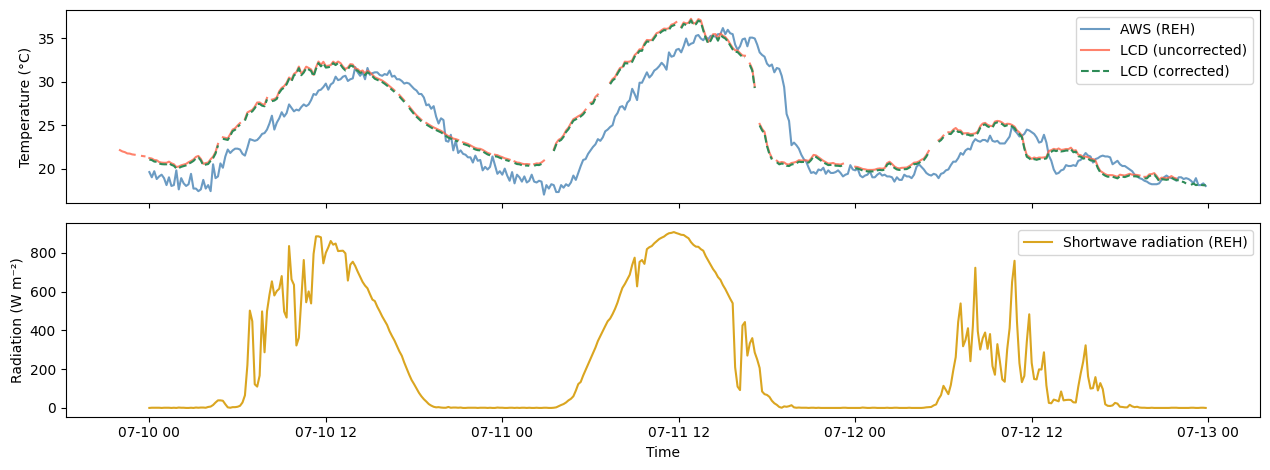
Results#

We can now inspect the correction for a LCD station over a three day window in mid-July alongside the shortwave radiation of the nearest MeteoSwiss reference, to assess the differences between AWS and LCD data (raw and corrected) as well as how these relate to the incoming shortwave radiation:

aws_wide = utils.long_to_wide(aws_ts_df)
station_id = lcd_ts_df.columns[0]
plot_slice = slice("2023-07-10", "2023-07-12")

rad_wide = aws_wide[settings.ECV_RADIATION_SHORTWAVE]
aws_temp_wide = aws_wide[settings.ECV_TEMPERATURE]
aws_station_id = rad_wide.columns[0]  # nearest AWS station (approximate)

fig, axes = plt.subplots(nrows=2, sharex=True, figsize=(2 * figwidth, figheight))

axes[0].plot(
    aws_temp_wide.loc[plot_slice, aws_station_id],
    label=f"AWS ({aws_station_id})",
    color="steelblue",
    alpha=0.8,
)
axes[0].plot(
    lcd_ts_df.loc[plot_slice, station_id],
    label="LCD (uncorrected)",
    color="tomato",
    alpha=0.8,
)
axes[0].plot(
    cor_ts_df.loc[plot_slice, station_id],
    label="LCD (corrected)",
    color="seagreen",
    linewidth=1.5,
    linestyle="--",
)
axes[0].set_ylabel("Temperature (\u00b0C)")
axes[0].legend()

axes[1].plot(
    rad_wide.loc[plot_slice, aws_station_id],
    color="goldenrod",
    label=f"Shortwave radiation ({aws_station_id})",
)
axes[1].set_ylabel("Radiation (W m\u207b\u00b2)")
axes[1].set_xlabel("Time")
axes[1].legend()

fig.tight_layout()

../_images/3adc90fb34b3a7ed8882e7b9ba0416a64f7275370c80342855b91f691445f282.png

Training a correction model#

Besides supporting the application of pre-trained models (i.e., via apply_bias_correction), meteora also supports training custom bias correction models given a paired time series of shortwave radiation from a co-located reference AWS (X_train) and the observed temperature bias at the LCD sensor (y_train, i.e. LCD minus reference temperature). For the most part, this is essentially done using scikit-learn’s pipelines, which is a sequence of data transformations with a final predictor model. We can actually inspect the structure of the pre-trained pipeline by loading it explicitly:

model = load_correction_model(repo_id, filename, trusted=trusted)
model

/home/docs/checkouts/readthedocs.org/user_builds/meteora/checkouts/stable/.pixi/envs/doc/lib/python3.13/site-packages/sklearn/base.py:463: InconsistentVersionWarning: Trying to unpickle estimator Pipeline from version 1.7.2 when using version 1.8.0. This might lead to breaking code or invalid results. Use at your own risk. For more info please refer to:
https://scikit-learn.org/stable/model_persistence.html#security-maintainability-limitations
  warnings.warn(

Pipeline(steps=[('radiation_transformer',
                 BestScaleRadiationTransformer(radiation_col='radiation_shortwave',
                                               time_col='time',
                                               window_minutes=[60, 120, 180,
                                                               240, 300])),
                ('model', ExplainableBoostingRegressor())])

In a Jupyter environment, please rerun this cell to show the HTML representation or trust the notebook.
On GitHub, the HTML representation is unable to render, please try loading this page with nbviewer.org.

We can see that the pipeline is composed of the BestScaleRadiationTransformer followed by an ExplainableBosstingRegressor (Lou et al., 2013, Nori et al., 2019). The BestScaleRadiationTransformer from meteora is based on the observation that the temperature bias of an unshielded sensor is driven not only by instantaneous shortwave radiation but also by its accumulation over preceding time (due to the thermal inertia of the sensor) (Beele et al., 2022, Bell et al., 2015, Cornes et al., 2020). Accordingly, the transformer evaluates a set of candidate rolling-sum windows (in minutes) and selects the one most correlated with the observed temperature bias during fit; transform then applies that window to a new radiation time series and returns the result as a single-column DataFrame ready for any scikit-learn-compatible regressor.

Below we illustrate the workflow with the MeteoSwiss radiation data and a synthetic bias of 3 mK per W m⁻²:

rad_ser = aws_wide[settings.ECV_RADIATION_SHORTWAVE].iloc[:, 0].dropna()

# X_train: time + radiation columns; y_train: temperature bias (LCD - reference)
# in practice y_train comes from paired LCD–reference measurements
X_train = pd.DataFrame(
    {
        settings.TIME_COL: rad_ser.index,
        settings.ECV_RADIATION_SHORTWAVE: rad_ser.values,
    }
)
y_train = (
    0.003 * rad_ser.values
)  # synthetic: 3 mK per W m\u207b\u00b2 (for illustration)

window_minutes = [30, 60, 120, 240]
pipeline = Pipeline(
    [
        ("transformer", BestScaleRadiationTransformer(window_minutes)),
        ("regressor", LinearRegression()),
    ]
)
pipeline.fit(X_train, y_train)
print(f"Best radiation window: {pipeline['transformer'].best_scale_} min")

---------------------------------------------------------------------------
ValueError                                Traceback (most recent call last)
Cell In[11], line 22
window_minutes = [30, 60, 120, 240]
pipeline = Pipeline(
   [
       ("transformer", BestScaleRadiationTransformer(window_minutes)),
       ("regressor", LinearRegression()),
   ]
)
---> 22 pipeline.fit(X_train, y_train)
print(f"Best radiation window: {pipeline['transformer'].best_scale_} min")

File ~/checkouts/readthedocs.org/user_builds/meteora/checkouts/stable/.pixi/envs/doc/lib/python3.13/site-packages/sklearn/base.py:1336, in _fit_context.<locals>.decorator.<locals>.wrapper(estimator, *args, **kwargs)
   estimator._validate_params()
with config_context(
   skip_parameter_validation=(
       prefer_skip_nested_validation or global_skip_validation
   )
):
-> 1336     return fit_method(estimator, *args, **kwargs)

File ~/checkouts/readthedocs.org/user_builds/meteora/checkouts/stable/.pixi/envs/doc/lib/python3.13/site-packages/sklearn/pipeline.py:621, in Pipeline.fit(self, X, y, **params)
   if self._final_estimator != "passthrough":
       last_step_params = self._get_metadata_for_step(
           step_idx=len(self) - 1,
           step_params=routed_params[self.steps[-1][0]],
           all_params=params,
       )
--> 621         self._final_estimator.fit(Xt, y, **last_step_params["fit"])
return self

File ~/checkouts/readthedocs.org/user_builds/meteora/checkouts/stable/.pixi/envs/doc/lib/python3.13/site-packages/sklearn/base.py:1336, in _fit_context.<locals>.decorator.<locals>.wrapper(estimator, *args, **kwargs)
   estimator._validate_params()
with config_context(
   skip_parameter_validation=(
       prefer_skip_nested_validation or global_skip_validation
   )
):
-> 1336     return fit_method(estimator, *args, **kwargs)

File ~/checkouts/readthedocs.org/user_builds/meteora/checkouts/stable/.pixi/envs/doc/lib/python3.13/site-packages/sklearn/linear_model/_base.py:630, in LinearRegression.fit(self, X, y, sample_weight)
n_jobs_ = self.n_jobs
accept_sparse = False if self.positive else ["csr", "csc", "coo"]
--> 630 X, y = validate_data(
   self,
   X,
   y,
   accept_sparse=accept_sparse,
   y_numeric=True,
   multi_output=True,
   force_writeable=True,
)
has_sw = sample_weight is not None
if has_sw:

File ~/checkouts/readthedocs.org/user_builds/meteora/checkouts/stable/.pixi/envs/doc/lib/python3.13/site-packages/sklearn/utils/validation.py:2919, in validate_data(_estimator, X, y, reset, validate_separately, skip_check_array, **check_params)
       y = check_array(y, input_name="y", **check_y_params)
   else:
-> 2919         X, y = check_X_y(X, y, **check_params)
   out = X, y
if not no_val_X and check_params.get("ensure_2d", True):

File ~/checkouts/readthedocs.org/user_builds/meteora/checkouts/stable/.pixi/envs/doc/lib/python3.13/site-packages/sklearn/utils/validation.py:1314, in check_X_y(X, y, accept_sparse, accept_large_sparse, dtype, order, copy, force_writeable, ensure_all_finite, ensure_2d, allow_nd, multi_output, ensure_min_samples, ensure_min_features, y_numeric, estimator)
       estimator_name = _check_estimator_name(estimator)
   raise ValueError(
       f"{estimator_name} requires y to be passed, but the target y is None"
   )
-> 1314 X = check_array(
   X,
   accept_sparse=accept_sparse,
   accept_large_sparse=accept_large_sparse,
   dtype=dtype,
   order=order,
   copy=copy,
   force_writeable=force_writeable,
   ensure_all_finite=ensure_all_finite,
   ensure_2d=ensure_2d,
   allow_nd=allow_nd,
   ensure_min_samples=ensure_min_samples,
   ensure_min_features=ensure_min_features,
   estimator=estimator,
   input_name="X",
)
y = _check_y(y, multi_output=multi_output, y_numeric=y_numeric, estimator=estimator)
check_consistent_length(X, y)

File ~/checkouts/readthedocs.org/user_builds/meteora/checkouts/stable/.pixi/envs/doc/lib/python3.13/site-packages/sklearn/utils/validation.py:1074, in check_array(array, accept_sparse, accept_large_sparse, dtype, order, copy, force_writeable, ensure_all_finite, ensure_non_negative, ensure_2d, allow_nd, ensure_min_samples, ensure_min_features, estimator, input_name)
   raise ValueError(
       f"Found array with dim {array.ndim},"
       f" while dim <= 2 is required{context}."
   )
if ensure_all_finite:
-> 1074     _assert_all_finite(
       array,
       input_name=input_name,
       estimator_name=estimator_name,
       allow_nan=ensure_all_finite == "allow-nan",
   )
if copy:
   if _is_numpy_namespace(xp):
       # only make a copy if `array` and `array_orig` may share memory`

File ~/checkouts/readthedocs.org/user_builds/meteora/checkouts/stable/.pixi/envs/doc/lib/python3.13/site-packages/sklearn/utils/validation.py:133, in _assert_all_finite(X, allow_nan, msg_dtype, estimator_name, input_name)
if first_pass_isfinite:
   return
--> 133 _assert_all_finite_element_wise(
   X,
   xp=xp,
   allow_nan=allow_nan,
   msg_dtype=msg_dtype,
   estimator_name=estimator_name,
   input_name=input_name,
)

File ~/checkouts/readthedocs.org/user_builds/meteora/checkouts/stable/.pixi/envs/doc/lib/python3.13/site-packages/sklearn/utils/validation.py:182, in _assert_all_finite_element_wise(X, xp, allow_nan, msg_dtype, estimator_name, input_name)
if estimator_name and input_name == "X" and has_nan_error:
   # Improve the error message on how to handle missing values in
   # scikit-learn.
   msg_err += (
       f"\n{estimator_name} does not accept missing values"
       " encoded as NaN natively. For supervised learning, you might want"
   (...)    180         "#estimators-that-handle-nan-values"
   )
--> 182 raise ValueError(msg_err)

ValueError: Input X contains NaN.
LinearRegression does not accept missing values encoded as NaN natively. For supervised learning, you might want to consider sklearn.ensemble.HistGradientBoostingClassifier and Regressor which accept missing values encoded as NaNs natively. Alternatively, it is possible to preprocess the data, for instance by using an imputer transformer in a pipeline or drop samples with missing values. See https://scikit-learn.org/stable/modules/impute.html You can find a list of all estimators that handle NaN values at the following page: https://scikit-learn.org/stable/modules/impute.html#estimators-that-handle-nan-values

While LinearRegression works well as a first-order approximation, non-linear models may better capture the relationship between accumulated radiation and sensor bias (Beele et al., 2022, Bosch and Burger, 2026, Cornes et al., 2020).

skops_io.dump(pipeline, "my-device.skops")

from huggingface_hub import HfApi

api = HfApi()
api.create_repo("username/lcd-bias-correction", repo_type="model", exist_ok=True)
api.upload_file(
    path_or_fileobj="my-device.skops",
    path_in_repo="my-device.skops",
    repo_id="username/lcd-bias-correction",
)

References#

[1] (1,2)

Eva Beele, Maarten Reyniers, Raf Aerts, and Ben Somers. Quality control and correction method for air temperature data from a citizen science weather station network in leuven, belgium. Earth System Science Data, 14(10):4681–4717, 2022.

[2] (1,2)

Simon Bell, Dan Cornford, and Lucy Bastin. How good are citizen weather stations? addressing a biased opinion. Weather, 70(3):75–84, 2015.

[3] (1,2,3)

Mart\'ı Bosch and Moritz Burger. Revisiting urban heat indices in switzerland using low-cost measurement networks. 2026. URL: https://arxiv.org/abs/2606.09364, arXiv:2606.09364.

[4]

Yann Georg Büchau. Modelling Shield Temperature Sensors: An Assessment of the Netatmo Citizen Weather Station. PhD thesis, Universität Hamburg, 2018.

[5]

Lee Chapman, Cassandra Bell, and Simon Bell. Can the crowdsourcing data paradigm take atmospheric science to a new level?: a case study of the urban heat island of london quantified using netatmo weather stations. International Journal of Climatology, 2016.

[6] (1,2,3)

Richard C Cornes, Marieke Dirksen, and Raymond Sluiter. Correcting citizen-science air temperature measurements across the netherlands for short wave radiation bias. Meteorological Applications, 27(1):e1814, 2020.

[7]

Yin Lou, Rich Caruana, Johannes Gehrke, and Giles Hooker. Accurate intelligible models with pairwise interactions. In Proceedings of the 19th ACM SIGKDD international conference on Knowledge discovery and data mining, 623–631. ACM, 2013.

[8]

C. Muller, L. Chapman, C. S. B. Grimmond, D. Young, and X. Cai. Sensors and the city: a review of urban meteorological networks. International Journal of Climatology, 33(7):1585–1600, 2013.

[9]

Harsha Nori, Samuel Jenkins, Paul Koch, and Rich Caruana. Interpretml: a unified framework for machine learning interpretability. arXiv preprint arXiv:1909.09223, 2019.

[10]

Carmen Hau Man Wong, Yu Ting Kwok, Yueyang He, and Edward Ng. Government-involved urban meteorological networks (umns): a global review. Urban Climate, 61:102409, 2025.

[11]

Amt für Abfall, Wasser, Energie und Luft. Lufttemperatur und luftfeuchte lora-sensor-messwerte. Available from (in German) https://opendata.swiss/de/dataset/lufttemperatur-und-luftfeuchte-lora-sensor-messwerte. Accessed: 14 January 2026, 2026.

	steps steps: list of tuples List of (name of step, estimator) tuples that are to be chained in sequential order. To be compatible with the scikit-learn API, all steps must define `fit`. All non-last steps must also define `transform`. See :ref:`Combining Estimators ` for more details.	[('radiation_transformer', ...), ('model', ...)]
	transform_input transform_input: list of str, default=None The names of the :term:`metadata` parameters that should be transformed by the pipeline before passing it to the step consuming it. This enables transforming some input arguments to ``fit`` (other than ``X``) to be transformed by the steps of the pipeline up to the step which requires them. Requirement is defined via :ref:`metadata routing `. For instance, this can be used to pass a validation set through the pipeline. You can only set this if metadata routing is enabled, which you can enable using ``sklearn.set_config(enable_metadata_routing=True)``. .. versionadded:: 1.6	None
	memory memory: str or object with the joblib.Memory interface, default=None Used to cache the fitted transformers of the pipeline. The last step will never be cached, even if it is a transformer. By default, no caching is performed. If a string is given, it is the path to the caching directory. Enabling caching triggers a clone of the transformers before fitting. Therefore, the transformer instance given to the pipeline cannot be inspected directly. Use the attribute ``named_steps`` or ``steps`` to inspect estimators within the pipeline. Caching the transformers is advantageous when fitting is time consuming. See :ref:`sphx_glr_auto_examples_neighbors_plot_caching_nearest_neighbors.py` for an example on how to enable caching.	None
	verbose verbose: bool, default=False If True, the time elapsed while fitting each step will be printed as it is completed.	False

	feature_names	None
	feature_types	None
	max_bins	1024
	max_interaction_bins	64
	interactions	'5x'
	exclude	None
	validation_size	0.15
	outer_bags	14
	inner_bags	0
	learning_rate	0.04
	greedy_ratio	10.0
	cyclic_progress	False
	smoothing_rounds	500
	interaction_smoothing_rounds	100
	max_rounds	50000
	early_stopping_rounds	100
	early_stopping_tolerance	1e-05
	callback	None
	min_samples_leaf	4
	min_hessian	0.0
	reg_alpha	0.0
	reg_lambda	0.0
	max_delta_step	0.0
	gain_scale	5.0
	min_cat_samples	10
	cat_smooth	10.0
	missing	'separate'
	max_leaves	2
	monotone_constraints	None
	objective	'rmse'
	n_jobs	-2
	random_state	42

	window_minutes	[60, 120, ...]
	time_col	'time'
	radiation_col	'radiation_shortwave'

Radiation bias correction for low-cost temperature sensors#

LCD sensor data#

Reference weather station data#

Applying bias correction#

Results#

Training a correction model#

References#

This Page