Data structures for geospatial time series data

import contextily as cx
import matplotlib.pyplot as plt
import osmnx as ox
import seaborn as sns
import xarray as xr

from meteora import clients, utils

region = "Switzerland"
start = "2021-08-13"
end = "2021-08-16"
variables = ["temperature", "precipitation", "wind_speed"]

client = clients.METARASOSIEMClient(region)

ts_df = client.get_ts_df(variables, start=start, end=end)
ts_df

		temperature	precipitation	wind_speed
station_id	time
LSGC	2021-08-13 00:20:00+00:00	60.8	0.0	1.0
	2021-08-13 00:50:00+00:00	60.8	0.0	2.0
	2021-08-13 01:20:00+00:00	60.8	0.0	2.0
	2021-08-13 01:50:00+00:00	59.0	0.0	0.0
	2021-08-13 02:20:00+00:00	59.0	0.0	0.0
...	...	...	...	...
LSZS	2021-08-15 21:50:00+00:00	51.8	0.0	4.0
	2021-08-15 22:20:00+00:00	51.8	0.0	2.0
	2021-08-15 22:50:00+00:00	51.8	0.0	4.0
	2021-08-15 23:20:00+00:00	50.0	0.0	2.0
	2021-08-15 23:50:00+00:00	50.0	0.0	1.0

2304 rows × 3 columns

There are different ways in which we can structure time series data frame shown above. The most common representation are the so-called long and wide table formats (see the “Data structures accepted by seaborn” section of the seaborn documentation for an overview).

Long data frames

The get_ts_df method returns a long data frame where the station and time are used as multi-index levels, so that we can easily select the time series of a specific station:

station_id = "LSGG"
ts_df.loc[station_id]

	temperature	precipitation	wind_speed
time
2021-08-13 00:20:00+00:00	64.4	0.0	4.0
2021-08-13 00:50:00+00:00	62.6	0.0	1.0
2021-08-13 01:20:00+00:00	62.6	0.0	3.0
2021-08-13 01:50:00+00:00	62.6	0.0	2.0
2021-08-13 02:20:00+00:00	62.6	0.0	3.0
...	...	...	...
2021-08-15 21:50:00+00:00	77.0	0.0	2.0
2021-08-15 22:20:00+00:00	77.0	0.0	4.0
2021-08-15 22:50:00+00:00	77.0	0.0	10.0
2021-08-15 23:20:00+00:00	68.0	0.0	7.0
2021-08-15 23:50:00+00:00	68.0	0.0	3.0

144 rows × 3 columns

The key advantage of a long data frame for time series data is that it is very flexible, i.e., we can combine stations with different time ranges and temporal resolutions into a single data frame structure. However, performing simple time series operations requires grouping by stations, which may not be the most convenient and straight-forward.

Wide data frames

The same data can be represented as a wide data frame, where the index is the time and the variables and stations are the multi-level columns. We can convert the long data frame to a wide data frame using the meteora.utils.long_to_wide function:

# in this case, equivalently:
# wide_ts_df = ts_df.unstack(level="station")
wide_ts_df = utils.long_to_wide(ts_df)
wide_ts_df

variable	temperature										...	wind_speed
station_id	LSGC	LSGG	LSGS	LSMA	LSMD	LSME	LSMM	LSMP	LSZA	LSZB	...	LSMM	LSMP	LSZA	LSZB	LSZC	LSZG	LSZH	LSZL	LSZR	LSZS
time
2021-08-13 00:20:00+00:00	60.8	64.4	64.4	69.8	68.0	69.8	66.2	68.0	71.6	64.4	...	2.0	4.0	8.0	3.0	4.0	2.0	7.0	5.0	6.0	1.0
2021-08-13 00:50:00+00:00	60.8	62.6	64.4	68.0	66.2	69.8	66.2	68.0	71.6	62.6	...	3.0	4.0	4.0	3.0	2.0	2.0	4.0	7.0	3.0	4.0
2021-08-13 01:20:00+00:00	60.8	62.6	64.4	66.2	60.8	68.0	64.4	68.0	71.6	62.6	...	4.0	3.0	2.0	1.0	2.0	2.0	5.0	8.0	6.0	2.0
2021-08-13 01:50:00+00:00	59.0	62.6	62.6	66.2	59.0	66.2	64.4	66.2	69.8	62.6	...	3.0	3.0	3.0	2.0	4.0	2.0	2.0	7.0	5.0	2.0
2021-08-13 02:20:00+00:00	59.0	62.6	62.6	64.4	59.0	64.4	62.6	64.4	69.8	62.6	...	3.0	0.0	4.0	2.0	3.0	2.0	4.0	3.0	4.0	1.0
...	...	...	...	...	...	...	...	...	...	...	...	...	...	...	...	...	...	...	...	...	...
2021-08-15 21:50:00+00:00	62.6	77.0	75.2	73.4	-4.0	75.2	69.8	71.6	75.2	68.0	...	0.0	1.0	1.0	1.0	2.0	1.0	2.0	3.0	2.0	4.0
2021-08-15 22:20:00+00:00	64.4	77.0	75.2	71.6	12.2	73.4	68.0	71.6	75.2	66.2	...	3.0	0.0	2.0	2.0	9.0	4.0	2.0	2.0	4.0	2.0
2021-08-15 22:50:00+00:00	66.2	77.0	75.2	69.8	-13.0	71.6	68.0	71.6	73.4	66.2	...	6.0	2.0	2.0	2.0	15.0	3.0	2.0	2.0	5.0	4.0
2021-08-15 23:20:00+00:00	64.4	68.0	75.2	71.6	26.6	71.6	68.0	75.2	75.2	66.2	...	3.0	3.0	3.0	4.0	9.0	3.0	2.0	2.0	5.0	2.0
2021-08-15 23:50:00+00:00	66.2	68.0	71.6	73.4	23.0	71.6	68.0	69.8	73.4	68.0	...	1.0	2.0	1.0	2.0	8.0	5.0	2.0	3.0	3.0	1.0

144 rows × 48 columns

Accordingly, we can easily select the time series of a specific variable:

wide_ts_df["temperature"]

station_id	LSGC	LSGG	LSGS	LSMA	LSMD	LSME	LSMM	LSMP	LSZA	LSZB	LSZC	LSZG	LSZH	LSZL	LSZR	LSZS
time
2021-08-13 00:20:00+00:00	60.8	64.4	64.4	69.8	68.0	69.8	66.2	68.0	71.6	64.4	68.0	68.0	71.6	71.6	71.6	50.0
2021-08-13 00:50:00+00:00	60.8	62.6	64.4	68.0	66.2	69.8	66.2	68.0	71.6	62.6	69.8	66.2	71.6	73.4	71.6	50.0
2021-08-13 01:20:00+00:00	60.8	62.6	64.4	66.2	60.8	68.0	64.4	68.0	71.6	62.6	68.0	66.2	69.8	73.4	73.4	50.0
2021-08-13 01:50:00+00:00	59.0	62.6	62.6	66.2	59.0	66.2	64.4	66.2	69.8	62.6	66.2	64.4	69.8	73.4	69.8	50.0
2021-08-13 02:20:00+00:00	59.0	62.6	62.6	64.4	59.0	64.4	62.6	64.4	69.8	62.6	68.0	62.6	69.8	73.4	71.6	48.2
...	...	...	...	...	...	...	...	...	...	...	...	...	...	...	...	...
2021-08-15 21:50:00+00:00	62.6	77.0	75.2	73.4	-4.0	75.2	69.8	71.6	75.2	68.0	73.4	71.6	71.6	73.4	73.4	51.8
2021-08-15 22:20:00+00:00	64.4	77.0	75.2	71.6	12.2	73.4	68.0	71.6	75.2	66.2	73.4	71.6	69.8	73.4	77.0	51.8
2021-08-15 22:50:00+00:00	66.2	77.0	75.2	69.8	-13.0	71.6	68.0	71.6	73.4	66.2	71.6	69.8	69.8	73.4	78.8	51.8
2021-08-15 23:20:00+00:00	64.4	68.0	75.2	71.6	26.6	71.6	68.0	75.2	75.2	66.2	73.4	71.6	69.8	73.4	78.8	50.0
2021-08-15 23:50:00+00:00	66.2	68.0	71.6	73.4	23.0	71.6	68.0	69.8	73.4	68.0	69.8	75.2	69.8	73.4	77.0	50.0

144 rows × 16 columns

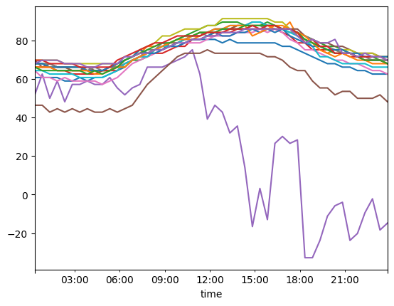
Note that unlike in the long data frame, the records of all the stations and variables are indexed by a common and unique timestamp. Accordingly, a key advantage of the wide data frame is that time series operations are supported by pandas out-of-the-box. For example, we can easily select a time range and plot the temperature time series of all stations:

wide_ts_df.loc["2021-08-14 00:00:00":"2021-08-15 00:00:00"]["temperature"].plot(
    legend=False
)

<Axes: xlabel='time'>

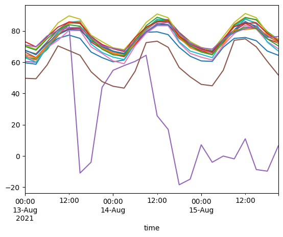
We can also resample the time series to a different frequency, e.g., we can compute the hourly mean temperature time series of all stations:

wide_ts_df.resample("3h")["temperature"].mean().plot(legend=False)

<Axes: xlabel='time'>

The main disadvantage is the wide data form may not be appropriate to store raw observations from different sources at different time resolutions, since it can result in many nan values.

Example geospatial operations with long and wide data frames

We have so far reviewed the advantages and disatvantages that the long and wide data frame forms feature when dealing with time series data. However, meteorological observations also have an important geospatial component which we have not addressed yet. While it is possible to add a “geometry” column to the long data frame, it would result in many repeated values (since we likely have many observations for each station). On the other hand, stations are featured as rows in the wide data frame, which makes adding their geolocation very inconvenient.

Therefore, in most cases the best way to peform spatial operations on meteorological data is to use two separate data structures, i.e., one for the time series of measurements and another with the station locations (and potentially other attributes). As shown above, the station locations can be accessed in the stations_gdf property, which we can use to perform geospatial operations. For example, we can select stations within a buffer around a specific location:

query = "Canton de Vaud"
buffer_dist = 20e3  # in meters

extent_geom = (
    ox.projection.project_gdf(ox.geocode_to_gdf(query))
    .buffer(buffer_dist)
    .to_crs(client.stations_gdf.crs)
    .iloc[0]
)
station_ids = client.stations_gdf[client.stations_gdf.within(extent_geom)].index
station_ids

Index(['LSGC', 'LSGG', 'LSGS', 'LSMP'], dtype='str', name='station_id')

We can use this information to select the time series of the stations within the buffer. For the long data frame (the default in Meteora), this is straightforward since the stations are the first-level index:

ts_df.loc[station_ids]

		temperature	precipitation	wind_speed
station_id	time
LSGC	2021-08-13 00:20:00+00:00	60.8	0.0	1.0
	2021-08-13 00:50:00+00:00	60.8	0.0	2.0
	2021-08-13 01:20:00+00:00	60.8	0.0	2.0
	2021-08-13 01:50:00+00:00	59.0	0.0	0.0
	2021-08-13 02:20:00+00:00	59.0	0.0	0.0
...	...	...	...	...
LSMP	2021-08-15 21:50:00+00:00	71.6	0.0	1.0
	2021-08-15 22:20:00+00:00	71.6	0.0	0.0
	2021-08-15 22:50:00+00:00	71.6	0.0	2.0
	2021-08-15 23:20:00+00:00	75.2	0.0	3.0
	2021-08-15 23:50:00+00:00	69.8	0.0	2.0

576 rows × 3 columns

For the wide data frame, stations are in the second level of the columns, so we can either (i) swap the column levels and then simply pass station_ids to select the desired stations or (ii) use .loc at the second level of the columns:

# (i)
# wide_ts_df.swaplevel("variable", "station", axis="columns")[station_ids]
# (ii)
wide_ts_df.loc[:, (slice(None), station_ids)]

variable	temperature				precipitation				wind_speed
station_id	LSGC	LSGG	LSGS	LSMP	LSGC	LSGG	LSGS	LSMP	LSGC	LSGG	LSGS	LSMP
time
2021-08-13 00:20:00+00:00	60.8	64.4	64.4	68.0	0.0	0.0	0.0	0.0	1.0	4.0	4.0	4.0
2021-08-13 00:50:00+00:00	60.8	62.6	64.4	68.0	0.0	0.0	0.0	0.0	2.0	1.0	5.0	4.0
2021-08-13 01:20:00+00:00	60.8	62.6	64.4	68.0	0.0	0.0	0.0	0.0	2.0	3.0	0.0	3.0
2021-08-13 01:50:00+00:00	59.0	62.6	62.6	66.2	0.0	0.0	0.0	0.0	0.0	2.0	0.0	3.0
2021-08-13 02:20:00+00:00	59.0	62.6	62.6	64.4	0.0	0.0	0.0	0.0	0.0	3.0	2.0	0.0
...	...	...	...	...	...	...	...	...	...	...	...	...
2021-08-15 21:50:00+00:00	62.6	77.0	75.2	71.6	0.0	0.0	0.0	0.0	1.0	2.0	3.0	1.0
2021-08-15 22:20:00+00:00	64.4	77.0	75.2	71.6	0.0	0.0	0.0	0.0	2.0	4.0	3.0	0.0
2021-08-15 22:50:00+00:00	66.2	77.0	75.2	71.6	0.0	0.0	0.0	0.0	5.0	10.0	3.0	2.0
2021-08-15 23:20:00+00:00	64.4	68.0	75.2	75.2	0.0	0.0	0.0	0.0	6.0	7.0	5.0	3.0
2021-08-15 23:50:00+00:00	66.2	68.0	71.6	69.8	0.0	0.0	0.0	0.0	6.0	3.0	1.0	2.0

144 rows × 12 columns

Note that if we are interested in a single variable, filtering by stations becomes much simpler:

wide_ts_df["temperature"][station_ids]

station_id	LSGC	LSGG	LSGS	LSMP
time
2021-08-13 00:20:00+00:00	60.8	64.4	64.4	68.0
2021-08-13 00:50:00+00:00	60.8	62.6	64.4	68.0
2021-08-13 01:20:00+00:00	60.8	62.6	64.4	68.0
2021-08-13 01:50:00+00:00	59.0	62.6	62.6	66.2
2021-08-13 02:20:00+00:00	59.0	62.6	62.6	64.4
...	...	...	...	...
2021-08-15 21:50:00+00:00	62.6	77.0	75.2	71.6
2021-08-15 22:20:00+00:00	64.4	77.0	75.2	71.6
2021-08-15 22:50:00+00:00	66.2	77.0	75.2	71.6
2021-08-15 23:20:00+00:00	64.4	68.0	75.2	75.2
2021-08-15 23:50:00+00:00	66.2	68.0	71.6	69.8

144 rows × 4 columns

Vector data cubes

As reviewed above, long and wide data frame forms have its own strengths and weaknesses when dealing with time series data, yet none of the forms offers a single object to encapsulate both the temporal and geospatial aspects of meteorological stations’ data. Luckily for us, there exists a data structure that fulfills our requirements - enter vector data cubes.

A vector data cube is an n-D array with at least one dimension indexed by vector geometries (Pebesma, 2022). In Python, this is represented as an xarray Dataset (or DataArray) object with an indexed dimension with vector geometries set using xvec. Given the time series data frame and station locations, we can get a vector data cube using the meteora.utils.long_to_cube function:

ts_cube = utils.long_to_cube(ts_df, client.stations_gdf)
ts_cube

<xarray.Dataset> Size: 57kB
Dimensions:        (geometry: 16, time: 144)
Coordinates:
  * geometry       (geometry) geometry 128B POINT (6.7928 47.0838) ... POINT ...
    station_id     (geometry) object 128B 'LSGC' 'LSGG' 'LSGS' ... 'LSZR' 'LSZS'
  * time           (time) datetime64[us, UTC] 1kB 2021-08-13 00:20:00+00:00 ....
Data variables:
    temperature    (geometry, time) float64 18kB 60.8 60.8 60.8 ... 50.0 50.0
    precipitation  (geometry, time) float64 18kB 0.0 0.0 0.0 0.0 ... 0.0 0.0 0.0
    wind_speed     (geometry, time) float64 18kB 1.0 2.0 2.0 0.0 ... 4.0 2.0 1.0
Indexes:
    geometry  GeometryIndex (crs=EPSG:4326)

xarray.Dataset

• Dimensions:
  • geometry: 16
  • time: 144
• Coordinates: (3)
  • geometry
    (geometry)
    geometry
    POINT (6.7928 47.0838) ... POINT...

    crs :

    EPSG:4326

    <GeometryArray>
    [<POINT (6.793 47.084)>, <POINT (6.128 46.248)>,  <POINT (7.33 46.219)>,
     <POINT (8.286 46.943)>,    <POINT (8.65 47.4)>, <POINT (8.305 47.092)>,
      <POINT (8.11 46.743)>, <POINT (6.942 46.812)>, <POINT (8.909 46.002)>,
     <POINT (7.497 46.914)>,   <POINT (8.38 46.97)>, <POINT (7.415 47.179)>,
      <POINT (8.53 47.478)>, <POINT (8.879 46.161)>, <POINT (9.561 47.485)>,
     <POINT (9.879 46.526)>]
    Length: 16, dtype: geometry

  • station_id
    (geometry)
    object
    'LSGC' 'LSGG' ... 'LSZR' 'LSZS'

    array(['LSGC', 'LSGG', 'LSGS', 'LSMA', 'LSMD', 'LSME', 'LSMM', 'LSMP', 'LSZA',
           'LSZB', 'LSZC', 'LSZG', 'LSZH', 'LSZL', 'LSZR', 'LSZS'], dtype=object)

  • time
    (time)
    datetime64[us, UTC]
    2021-08-13 00:20:00+00:00 ... 20...

    <DatetimeArray>
    ['2021-08-13 00:20:00+00:00', '2021-08-13 00:50:00+00:00',
     '2021-08-13 01:20:00+00:00', '2021-08-13 01:50:00+00:00',
     '2021-08-13 02:20:00+00:00', '2021-08-13 02:50:00+00:00',
     '2021-08-13 03:20:00+00:00', '2021-08-13 03:50:00+00:00',
     '2021-08-13 04:20:00+00:00', '2021-08-13 04:50:00+00:00',
     ...
     '2021-08-15 19:20:00+00:00', '2021-08-15 19:50:00+00:00',
     '2021-08-15 20:20:00+00:00', '2021-08-15 20:50:00+00:00',
     '2021-08-15 21:20:00+00:00', '2021-08-15 21:50:00+00:00',
     '2021-08-15 22:20:00+00:00', '2021-08-15 22:50:00+00:00',
     '2021-08-15 23:20:00+00:00', '2021-08-15 23:50:00+00:00']
    Length: 144, dtype: datetime64[us, UTC]

• Data variables: (3)
  • temperature
    (geometry, time)
    float64
    60.8 60.8 60.8 ... 51.8 50.0 50.0

    array([[60.8, 60.8, 60.8, ..., 66.2, 64.4, 66.2],
           [64.4, 62.6, 62.6, ..., 77. , 68. , 68. ],
           [64.4, 64.4, 64.4, ..., 75.2, 75.2, 71.6],
           ...,
           [71.6, 73.4, 73.4, ..., 73.4, 73.4, 73.4],
           [71.6, 71.6, 73.4, ..., 78.8, 78.8, 77. ],
           [50. , 50. , 50. , ..., 51.8, 50. , 50. ]], shape=(16, 144))

  • precipitation
    (geometry, time)
    float64
    0.0 0.0 0.0 0.0 ... 0.0 0.0 0.0 0.0

    array([[0., 0., 0., ..., 0., 0., 0.],
           [0., 0., 0., ..., 0., 0., 0.],
           [0., 0., 0., ..., 0., 0., 0.],
           ...,
           [0., 0., 0., ..., 0., 0., 0.],
           [0., 0., 0., ..., 0., 0., 0.],
           [0., 0., 0., ..., 0., 0., 0.]], shape=(16, 144))

  • wind_speed
    (geometry, time)
    float64
    1.0 2.0 2.0 0.0 ... 2.0 4.0 2.0 1.0

    array([[ 1.,  2.,  2., ...,  5.,  6.,  6.],
           [ 4.,  1.,  3., ..., 10.,  7.,  3.],
           [ 4.,  5.,  0., ...,  3.,  5.,  1.],
           ...,
           [ 5.,  7.,  8., ...,  2.,  2.,  3.],
           [ 6.,  3.,  6., ...,  5.,  5.,  3.],
           [ 1.,  4.,  2., ...,  4.,  2.,  1.]], shape=(16, 144))

• Indexes: (1)
  • geometry
    GeometryIndex (crs=EPSG:4326)

    GeometryIndex(
        [<POINT (6.793 47.084)>
         <POINT (6.128 46.248)>
         <POINT (7.33 46.219)>
         <POINT (8.286 46.943)>
         ...
         <POINT (8.53 47.478)>
         <POINT (8.879 46.161)>
         <POINT (9.561 47.485)>
         <POINT (9.879 46.526)>],
        crs=EPSG:4326)

We obtain an xarray Dataset with both the temporal and geospatial (respectively labeled as “time” and “station_id” following ts_df) coordinates and the three variables as data variables. Additionally, note in the “Indexes” section that the “station” index have the geospatial features enabled by xvec (note the GeometryIndex with the CRS).

The major advantage of vector data cubes is that we can now natively perform both time series and geospatial operations using a single object:

ts_cube["temperature"].sel(geometry=extent_geom, method="intersects").sel(
    time=slice("2021-08-13 12:00:00", "2021-08-14 12:00:00")
).resample(time="3h").mean()

<xarray.DataArray 'temperature' (geometry: 4, time: 8)> Size: 256B
array([[85.1, 84.8, 76.4, 70.7, 67.1, 65. , 71.6, 83.3],
       [81.5, 82.4, 74.9, 69.5, 65.9, 65. , 74.6, 80.6],
       [84.8, 85.4, 77. , 70.1, 67.1, 65.6, 73.1, 80.9],
       [77.3, 75.2, 66.5, 62.9, 60.2, 61.4, 71.9, 79.1]])
Coordinates:
  * geometry    (geometry) geometry 32B POINT (7.3303 46.2186) ... POINT (6.7...
    station_id  (geometry) object 32B 'LSGS' 'LSGG' 'LSMP' 'LSGC'
  * time        (time) datetime64[us, UTC] 64B 2021-08-13 12:00:00+00:00 ... ...
Indexes:
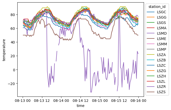
    geometry  GeometryIndex (crs=EPSG:4326)

xarray.DataArray

'temperature'

• geometry: 4
• time: 8

• 85.1 84.8 76.4 70.7 67.1 65.0 71.6 ... 66.5 62.9 60.2 61.4 71.9 79.1

  array([[85.1, 84.8, 76.4, 70.7, 67.1, 65. , 71.6, 83.3],
         [81.5, 82.4, 74.9, 69.5, 65.9, 65. , 74.6, 80.6],
         [84.8, 85.4, 77. , 70.1, 67.1, 65.6, 73.1, 80.9],
         [77.3, 75.2, 66.5, 62.9, 60.2, 61.4, 71.9, 79.1]])

• Coordinates: (3)
  • geometry
    (geometry)
    geometry
    POINT (7.3303 46.2186) ... POINT...

    crs :

    EPSG:4326

    <GeometryArray>
    [ <POINT (7.33 46.219)>, <POINT (6.128 46.248)>, <POINT (6.942 46.812)>,
     <POINT (6.793 47.084)>]
    Length: 4, dtype: geometry

  • station_id
    (geometry)
    object
    'LSGS' 'LSGG' 'LSMP' 'LSGC'

    array(['LSGS', 'LSGG', 'LSMP', 'LSGC'], dtype=object)

  • time
    (time)
    datetime64[us, UTC]
    2021-08-13 12:00:00+00:00 ... 20...

    <DatetimeArray>
    ['2021-08-13 12:00:00+00:00', '2021-08-13 15:00:00+00:00',
     '2021-08-13 18:00:00+00:00', '2021-08-13 21:00:00+00:00',
     '2021-08-14 00:00:00+00:00', '2021-08-14 03:00:00+00:00',
     '2021-08-14 06:00:00+00:00', '2021-08-14 09:00:00+00:00']
    Length: 8, dtype: datetime64[us, UTC]

• Indexes: (2)
  • geometry
    GeometryIndex (crs=EPSG:4326)

    GeometryIndex(
        [<POINT (7.33 46.219)>
         <POINT (6.128 46.248)>
         <POINT (6.942 46.812)>
         <POINT (6.793 47.084)>],
        crs=EPSG:4326)

  • time
    PandasIndex

    PandasIndex(DatetimeIndex(['2021-08-13 12:00:00+00:00', '2021-08-13 15:00:00+00:00',
                   '2021-08-13 18:00:00+00:00', '2021-08-13 21:00:00+00:00',
                   '2021-08-14 00:00:00+00:00', '2021-08-14 03:00:00+00:00',
                   '2021-08-14 06:00:00+00:00', '2021-08-14 09:00:00+00:00'],
                  dtype='datetime64[us, UTC]', name='time', freq='3h'))

We can also use the xvec accessor to plot our results, both in terms of time series data:

# assign_coords(station=ts_df.index.get_level_values("station").unique())
fig, ax = plt.subplots()
ts_cube["temperature"].plot.line(x="time", hue="station_id", add_legend=True, ax=ax)
sns.move_legend(ax, loc="center left", bbox_to_anchor=(1, 0.5))

or including geospatial information as well, e.g., stations colored by temperature averaged over a given period:

fig, ax = (
    ts_cube["temperature"]
    .sel(geometry=extent_geom, method="intersects")
    .sel(time=slice("2021-08-13 12:00:00", "2021-08-14 12:00:00"))
    .mean("time")
    .xvec.plot(cmap="coolwarm", geometry="geometry")
)
cx.add_basemap(ax, crs=ts_cube.geometry.crs, attribution=False)

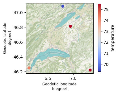
(C) OpenStreetMap contributors, Tiles style by Humanitarian OpenStreetMap Team hosted by OpenStreetMap France

StationBench format

The vector data cube is very similar to the ground truth station data format expected by StationBench to benchmark weather forecasts. The only differences are that instead of point geometry objects we have longitude/latitude coordinates (so geospatial operations are not enabled) and the variables use specific naming conventions. You can convert the long time series data frame to the expected xarray using the meteora.utils.long_to_stationbench function:

ts_ds = utils.long_to_stationbench(ts_df, client.stations_gdf)
ts_ds

<xarray.Dataset> Size: 57kB
Dimensions:         (time: 144, station_id: 16)
Coordinates:
  * time            (time) datetime64[us, UTC] 1kB 2021-08-13 00:20:00+00:00 ...
  * station_id      (station_id) object 128B 'LSGC' 'LSGG' ... 'LSZR' 'LSZS'
    longitude       (station_id) float64 128B 6.793 6.128 7.33 ... 9.561 9.879
    latitude        (station_id) float64 128B 47.08 46.25 46.22 ... 47.48 46.53
Data variables:
    2m_temperature  (time, station_id) float64 18kB 60.8 64.4 64.4 ... 77.0 50.0
    precipitation   (time, station_id) float64 18kB 0.0 0.0 0.0 ... 0.0 0.0 0.0
    10m_wind_speed  (time, station_id) float64 18kB 1.0 4.0 4.0 ... 3.0 3.0 1.0

xarray.Dataset

• Dimensions:
  • time: 144
  • station_id: 16
• Coordinates: (4)
  • time
    (time)
    datetime64[us, UTC]
    2021-08-13 00:20:00+00:00 ... 20...

    <DatetimeArray>
    ['2021-08-13 00:20:00+00:00', '2021-08-13 00:50:00+00:00',
     '2021-08-13 01:20:00+00:00', '2021-08-13 01:50:00+00:00',
     '2021-08-13 02:20:00+00:00', '2021-08-13 02:50:00+00:00',
     '2021-08-13 03:20:00+00:00', '2021-08-13 03:50:00+00:00',
     '2021-08-13 04:20:00+00:00', '2021-08-13 04:50:00+00:00',
     ...
     '2021-08-15 19:20:00+00:00', '2021-08-15 19:50:00+00:00',
     '2021-08-15 20:20:00+00:00', '2021-08-15 20:50:00+00:00',
     '2021-08-15 21:20:00+00:00', '2021-08-15 21:50:00+00:00',
     '2021-08-15 22:20:00+00:00', '2021-08-15 22:50:00+00:00',
     '2021-08-15 23:20:00+00:00', '2021-08-15 23:50:00+00:00']
    Length: 144, dtype: datetime64[us, UTC]

  • station_id
    (station_id)
    object
    'LSGC' 'LSGG' ... 'LSZR' 'LSZS'

    array(['LSGC', 'LSGG', 'LSGS', 'LSMA', 'LSMD', 'LSME', 'LSMM', 'LSMP', 'LSZA',
           'LSZB', 'LSZC', 'LSZG', 'LSZH', 'LSZL', 'LSZR', 'LSZS'], dtype=object)

  • longitude
    (station_id)
    float64
    6.793 6.128 7.33 ... 9.561 9.879

    array([6.7928, 6.1278, 7.3303, 8.2858, 8.65  , 8.3051, 8.11  , 6.9424,
           8.9092, 7.4972, 8.38  , 7.4151, 8.5302, 8.8786, 9.5608, 9.8789])

  • latitude
    (station_id)
    float64
    47.08 46.25 46.22 ... 47.48 46.53

    array([47.0838, 46.2475, 46.2186, 46.9431, 47.4   , 47.0924, 46.7433,
           46.8116, 46.0015, 46.9141, 46.97  , 47.1791, 47.4784, 46.1608,
           47.485 , 46.5264])

• Data variables: (3)
  • 2m_temperature
    (time, station_id)
    float64
    60.8 64.4 64.4 ... 73.4 77.0 50.0

    array([[60.8, 64.4, 64.4, ..., 71.6, 71.6, 50. ],
           [60.8, 62.6, 64.4, ..., 73.4, 71.6, 50. ],
           [60.8, 62.6, 64.4, ..., 73.4, 73.4, 50. ],
           ...,
           [66.2, 77. , 75.2, ..., 73.4, 78.8, 51.8],
           [64.4, 68. , 75.2, ..., 73.4, 78.8, 50. ],
           [66.2, 68. , 71.6, ..., 73.4, 77. , 50. ]], shape=(144, 16))

  • precipitation
    (time, station_id)
    float64
    0.0 0.0 0.0 0.0 ... 0.0 0.0 0.0 0.0

    array([[0., 0., 0., ..., 0., 0., 0.],
           [0., 0., 0., ..., 0., 0., 0.],
           [0., 0., 0., ..., 0., 0., 0.],
           ...,
           [0., 0., 0., ..., 0., 0., 0.],
           [0., 0., 0., ..., 0., 0., 0.],
           [0., 0., 0., ..., 0., 0., 0.]], shape=(144, 16))

  • 10m_wind_speed
    (time, station_id)
    float64
    1.0 4.0 4.0 1.0 ... 2.0 3.0 3.0 1.0

    array([[ 1.,  4.,  4., ...,  5.,  6.,  1.],
           [ 2.,  1.,  5., ...,  7.,  3.,  4.],
           [ 2.,  3.,  0., ...,  8.,  6.,  2.],
           ...,
           [ 5., 10.,  3., ...,  2.,  5.,  4.],
           [ 6.,  7.,  5., ...,  2.,  5.,  2.],
           [ 6.,  3.,  1., ...,  3.,  3.,  1.]], shape=(144, 16))

Saving to disk

There are several ways in which we can store the geospatial time series data that we deal with when using Meteora.

Using long or wide data frames

When using long and wide data frames, the most straight-forward solution is to separately save the stations geo-data frame and time series data frame to disk, e.g., using a geospatial file format for the former and a pandas data frame compatible format (CSV, JSON…) for the latter:

ts_df.to_csv("ts-df.csv")
client.stations_gdf.to_file("stations.gpkg")

Note that for long data frames, it is possible to save a single object by adding the station attributes as columns, however note that in most cases this will be highly inefficient and result in many repeated values.

For large amounts of data, you may consider tstore, which is an interoperable specification based on Apache Parquet and GeoParquet. (note that the API is still experimental). The first tutorial illustrates different ways in which long data frames from Meteora can be efficiently$^1$ stored while keeping the geospatial information.

Using vector data cubes

There exist several ways of saving vector data cubes to disk, which include (see the related section of the xvec documentation for more details):

• geospatial file formats, which is essentially equivalent to transforming the vector data cube to a long data frame with the station attributes (including location), and thus has the exact same shortcomings in terms of the high degree of repetition.

• binary serialization formats such as pickle and joblib, which have the advantage of allowing compression but may only work when read in a similar environment with similar package versions (therefore with restricted interoperability).

• CF conventions with netCDF or zarr, which encode the geospatial information so that it is compatible with the xarray’s formats such as netCDF and zarr.

Overall, the latter option is likely the most convenient. Let us try it (note that in order to run the cells below, we need to install zarr which is not a Meteora - nor xvec - dependency):

encoded = ts_cube.xvec.encode_cf()
# encoded.to_netcdf("geo-encoded.nc", mode="w")
encoded.to_zarr("geo-encoded.zarr", mode="w")

---------------------------------------------------------------------------
TypeError                                 Traceback (most recent call last)
Cell In[20], line 3
      1 encoded = ts_cube.xvec.encode_cf()
      2 # encoded.to_netcdf("geo-encoded.nc", mode="w")
----> 3 encoded.to_zarr("geo-encoded.zarr", mode="w")

File ~/checkouts/readthedocs.org/user_builds/meteora/checkouts/stable/.pixi/envs/doc/lib/python3.13/site-packages/xarray/core/dataset.py:2390, in Dataset.to_zarr(self, store, chunk_store, mode, synchronizer, group, encoding, compute, consolidated, append_dim, region, safe_chunks, align_chunks, storage_options, zarr_version, zarr_format, write_empty_chunks, chunkmanager_store_kwargs)
   2207 """Write dataset contents to a zarr group.
   2208 
   2209 Zarr chunks are determined in the following way:
   (...)   2386     The I/O user guide, with more details and examples.
   2387 """
   2388 from xarray.backends.writers import to_zarr
-> 2390 return to_zarr(  # type: ignore[call-overload,misc]
   2391     self,
   2392     store=store,
   2393     chunk_store=chunk_store,
   2394     storage_options=storage_options,
   2395     mode=mode,
   2396     synchronizer=synchronizer,
   2397     group=group,
   2398     encoding=encoding,
   2399     compute=compute,
   2400     consolidated=consolidated,
   2401     append_dim=append_dim,
   2402     region=region,
   2403     safe_chunks=safe_chunks,
   2404     align_chunks=align_chunks,
   2405     zarr_version=zarr_version,
   2406     zarr_format=zarr_format,
   2407     write_empty_chunks=write_empty_chunks,
   2408     chunkmanager_store_kwargs=chunkmanager_store_kwargs,
   2409 )

File ~/checkouts/readthedocs.org/user_builds/meteora/checkouts/stable/.pixi/envs/doc/lib/python3.13/site-packages/xarray/backends/writers.py:797, in to_zarr(dataset, store, chunk_store, mode, synchronizer, group, encoding, compute, consolidated, append_dim, region, safe_chunks, align_chunks, storage_options, zarr_version, zarr_format, write_empty_chunks, chunkmanager_store_kwargs)
    795 # TODO: figure out how to properly handle unlimited_dims
    796 try:
--> 797     dump_to_store(dataset, zstore, writer, encoding=encoding)
    798     writes = writer.sync(
    799         compute=compute, chunkmanager_store_kwargs=chunkmanager_store_kwargs
    800     )
    801 finally:

File ~/checkouts/readthedocs.org/user_builds/meteora/checkouts/stable/.pixi/envs/doc/lib/python3.13/site-packages/xarray/backends/writers.py:491, in dump_to_store(dataset, store, writer, encoder, encoding, unlimited_dims)
    488 if encoder:
    489     variables, attrs = encoder(variables, attrs)
--> 491 store.store(variables, attrs, check_encoding, writer, unlimited_dims=unlimited_dims)

File ~/checkouts/readthedocs.org/user_builds/meteora/checkouts/stable/.pixi/envs/doc/lib/python3.13/site-packages/xarray/backends/zarr.py:1009, in ZarrStore.store(self, variables, attributes, check_encoding_set, writer, unlimited_dims)
   1003     if self._append_dim not in existing_dims:
   1004         raise ValueError(
   1005             f"append_dim={self._append_dim!r} does not match any existing "
   1006             f"dataset dimensions {existing_dims}"
   1007         )
-> 1009 variables_encoded, attributes = self.encode(
   1010     {vn: variables[vn] for vn in new_variable_names}, attributes
   1011 )
   1013 if existing_variable_names:
   1014     # We make sure that values to be appended are encoded *exactly*
   1015     # as the current values in the store.
   1016     # To do so, we decode variables directly to access the proper encoding,
   1017     # without going via xarray.Dataset to avoid needing to load
   1018     # index variables into memory.
   1019     existing_vars, _, _ = conventions.decode_cf_variables(
   1020         variables={
   1021             k: self.open_store_variable(name=k) for k in existing_variable_names
   (...)   1025         attributes={},
   1026     )

File ~/checkouts/readthedocs.org/user_builds/meteora/checkouts/stable/.pixi/envs/doc/lib/python3.13/site-packages/xarray/backends/common.py:454, in AbstractWritableDataStore.encode(self, variables, attributes)
    452 for k, v in variables.items():
    453     try:
--> 454         encoded_variables[k] = self.encode_variable(v)
    455     except Exception as e:
    456         e.add_note(f"Raised while encoding variable {k!r} with value {v!r}")

File ~/checkouts/readthedocs.org/user_builds/meteora/checkouts/stable/.pixi/envs/doc/lib/python3.13/site-packages/xarray/backends/zarr.py:933, in ZarrStore.encode_variable(self, variable, name)
    932 def encode_variable(self, variable, name=None):
--> 933     variable = encode_zarr_variable(variable, name=name)
    934     return variable

File ~/checkouts/readthedocs.org/user_builds/meteora/checkouts/stable/.pixi/envs/doc/lib/python3.13/site-packages/xarray/backends/zarr.py:516, in encode_zarr_variable(var, needs_copy, name)
    495 def encode_zarr_variable(var, needs_copy=True, name=None):
    496     """
    497     Converts a Variable into another Variable which follows some
    498     of the CF conventions:
   (...)    513         A variable which has been encoded as described above.
    514     """
--> 516     var = conventions.encode_cf_variable(var, name=name)
    517     var = ensure_dtype_not_object(var, name=name)
    519     # zarr allows unicode, but not variable-length strings, so it's both
    520     # simpler and more compact to always encode as UTF-8 explicitly.
    521     # TODO: allow toggling this explicitly via dtype in encoding.
    522     # TODO: revisit this now that Zarr _does_ allow variable-length strings

File ~/checkouts/readthedocs.org/user_builds/meteora/checkouts/stable/.pixi/envs/doc/lib/python3.13/site-packages/xarray/conventions.py:102, in encode_cf_variable(var, needs_copy, name)
     90 ensure_not_multiindex(var, name=name)
     92 for coder in [
     93     CFDatetimeCoder(),
     94     CFTimedeltaCoder(),
   (...)    100     variables.BooleanCoder(),
    101 ]:
--> 102     var = coder.encode(var, name=name)
    104 for attr_name in CF_RELATED_DATA:
    105     pop_to(var.encoding, var.attrs, attr_name)

File ~/checkouts/readthedocs.org/user_builds/meteora/checkouts/stable/.pixi/envs/doc/lib/python3.13/site-packages/xarray/coding/times.py:1384, in CFDatetimeCoder.encode(self, variable, name)
   1383 def encode(self, variable: Variable, name: T_Name = None) -> Variable:
-> 1384     if np.issubdtype(variable.dtype, np.datetime64) or contains_cftime_datetimes(
   1385         variable
   1386     ):
   1387         dims, data, attrs, encoding = unpack_for_encoding(variable)
   1389         units = encoding.pop("units", None)

File ~/checkouts/readthedocs.org/user_builds/meteora/checkouts/stable/.pixi/envs/doc/lib/python3.13/site-packages/numpy/_core/numerictypes.py:534, in issubdtype(arg1, arg2)
    477 r"""
    478 Returns True if first argument is a typecode lower/equal in type hierarchy.
    479 
   (...)    531 
    532 """
    533 if not issubclass_(arg1, generic):
--> 534     arg1 = dtype(arg1).type
    535 if not issubclass_(arg2, generic):
    536     arg2 = dtype(arg2).type

TypeError: Cannot interpret 'datetime64[us, UTC]' as a data type
Raised while encoding variable 'time' with value <xarray.IndexVariable 'time' (time: 144)> Size: 1kB
<DatetimeArray>
['2021-08-13 00:20:00+00:00', '2021-08-13 00:50:00+00:00',
 '2021-08-13 01:20:00+00:00', '2021-08-13 01:50:00+00:00',
 '2021-08-13 02:20:00+00:00', '2021-08-13 02:50:00+00:00',
 '2021-08-13 03:20:00+00:00', '2021-08-13 03:50:00+00:00',
 '2021-08-13 04:20:00+00:00', '2021-08-13 04:50:00+00:00',
 ...
 '2021-08-15 19:20:00+00:00', '2021-08-15 19:50:00+00:00',
 '2021-08-15 20:20:00+00:00', '2021-08-15 20:50:00+00:00',
 '2021-08-15 21:20:00+00:00', '2021-08-15 21:50:00+00:00',
 '2021-08-15 22:20:00+00:00', '2021-08-15 22:50:00+00:00',
 '2021-08-15 23:20:00+00:00', '2021-08-15 23:50:00+00:00']
Length: 144, dtype: datetime64[us, UTC]

We can now read back the saved zarr store from disk into a vector data cube:

roundtripped = xr.open_zarr("geo-encoded.zarr").xvec.decode_cf()
roundtripped

which we can test to be identical to the original ts_cube (this may currently fail due to xvec/issues/141):

roundtripped.identical(ts_cube)

Footnotes

1. See a benchmark comparing tstore, netCDF and zarr in terms of resulting file sizes as well as reading and writing times.

References

[1]

Edzer Pebesma. Vector data cubes. r-spatial.org blog, 2022. URL: https://r-spatial.org/r/2022/09/12/vdc.html.