Overview#

This example notebook showcases the main features of Meteora. To that end, we will download and process meteorological observations from the Automated Surface/Weather Observing Systems (ASOS/AWOS) program, which comprises more than 900 automated weather stations in the United States.

More precisely, we will use the METARASOSIEMClient to stream METAR from the Iowa Environmental Mesonet.

import contextily as cx

from meteora import clients, climate_indices, settings, units

Meteora clients#

Meteora is essentially a collection of “client” classes that allow processing data from different providers in a standardized interface. The following sections will go through the main aspects of a Meteora client.

Selecting the client’s region of interest#

All clients are instantiated with at least the region argument, which defines the spatial extent of the required data. The region argument uses the pyregeon library and can be either:

A string with a place name (Nominatim query) to geocode.
A sequence with the west, south, east and north bounds.
A geometric object, e.g., shapely geometry, or a sequence of geometric objects. In such a case, the region will be passed as the data argument of the GeoSeries constructor.
A geopandas geo-series or geo-data frame.
A filename or URL, a file-like object opened in binary ('rb') mode, or a Path object that will be passed to geopandas.read_file.

In this case, we will use the country of Switzerland as defined by a query to the Nominatim API (via osmnx):

region = "Switzerland"

We can now instantiate our client:

client = clients.METARASOSIEMClient(region)

Stations locations and metadata#

The list of stations maintained by the provider within the selected region can be accessed using the stations_gdf property:

client.stations_gdf.head()

	elevation	sname	time_domain	archive_begin	archive_end	state	country	climate_site	wfo	tzname	...	ncei91	ugc_county	ugc_zone	county	sid	network	online	synop	attributes	geometry
station_id
LSGC	1027.0	Les Eplatures	(2001-Now)	2001-07-21	NaT	NaN	CH	NaN	NaN	Europe/Zurich	...	NaN	NaN	NaN	NaN	LSGC	CH__ASOS	True	99999.0	{'METAR_RESET_MINUTE': '50', 'GHCNH_ID': 'SZI0...	POINT (6.7928 47.0838)
LSGG	416.0	Geneva	(1935-Now)	1935-01-01	NaT	NaN	CH	NaN	NaN	Europe/Zurich	...	NaN	NaN	NaN	NaN	LSGG	CH__ASOS	True	99999.0	{'METAR_RESET_MINUTE': '50', 'GHCNH_ID': 'SZI0...	POINT (6.1278 46.2475)
LSGS	481.0	Sion	(1954-Now)	1954-12-31	NaT	NaN	CH	NaN	NaN	Europe/Zurich	...	NaN	NaN	NaN	NaN	LSGS	CH__ASOS	True	99999.0	{'METAR_RESET_MINUTE': '50', 'GHCNH_ID': 'SZI0...	POINT (7.3303 46.2186)
LSMA	444.0	Alpnach	(1977-Now)	1977-12-12	NaT	NaN	CH	NaN	NaN	Europe/Zurich	...	NaN	NaN	NaN	NaN	LSMA	CH__ASOS	True	99999.0	{'METAR_RESET_MINUTE': '50', 'GHCNH_ID': 'SZI0...	POINT (8.2858 46.9431)
LSMD	448.0	Dubendorf	(2004-Now)	2004-09-03	NaT	NaN	CH	NaN	NaN	Europe/Zurich	...	NaN	NaN	NaN	NaN	LSMD	CH__ASOS	True	99999.0	{'METAR_RESET_MINUTE': '50', 'GHCNH_ID': 'SZI0...	POINT (8.65 47.4)

5 rows × 21 columns

which is essentially a geopandas data frame that includes station metadata including the location, so we can, e.g., plot it in a map:

ax = client.stations_gdf.plot()
cx.add_basemap(ax, crs=client.stations_gdf.crs, attribution=False)

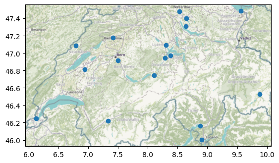
../_images/bfc559f32617b42fe7c92bab55b9f84a191df668073ae30d1da40cb94776b072.png

(C) OpenStreetMap contributors, Tiles style by Humanitarian OpenStreetMap Team hosted by OpenStreetMap France

Variables#

The list of variables and their metadata is shown in the variables_df property:

client.variables_df

	code	description
0	tmpf	Air Temperature
1	dwpf	Dew Point Temperature
2	relh	Relative Humidity
3	sknt	Wind Speed
4	drct	Wind Direction
5	mslp	Sea Level Pressure in millibar
6	p01i	1 minute precip

Getting a time series of measurements#

Given a list of variables and time range, we can use the get_ts_df method to get a time series of station measurements:

variables = ["tmpf", "dwpf", "relh"]
start = "2021-08-13"
end = "2021-08-16"

ts_df = client.get_ts_df(variables, start=start, end=end)
ts_df

		tmpf	dwpf	relh
station_id	time
LSGC	2021-08-13 00:20:00	60.8	53.6	77.14
	2021-08-13 00:50:00	60.8	53.6	77.14
	2021-08-13 01:20:00	60.8	53.6	77.14
	2021-08-13 01:50:00	59.0	53.6	82.25
	2021-08-13 02:20:00	59.0	53.6	82.25
...	...	...	...	...
LSZS	2021-08-15 21:50:00	51.8	48.2	87.47
	2021-08-15 22:20:00	51.8	48.2	87.47
	2021-08-15 22:50:00	51.8	48.2	87.47
	2021-08-15 23:20:00	50.0	46.4	87.37
	2021-08-15 23:50:00	50.0	46.4	87.37

2304 rows × 3 columns

Selecting date range#

While some providers only allow access to the most recent data, e.g., latest 24 hours, others allow querying data for a specific date range. In the latter case, the start and end arguments can be used to select the date range, which can be any object that can be converted to a pandas Timestamp object, i.e., a string, integer, float or a datetime object from the datetime module or numpy.

Selecting variables#

When accessing to time series data (e.g., the get_ts_df method of each client), the variables argument is used to select the variables to retrieve. The variables argument can be either:

a string or integer with variable name or code according to the provider’s nomenclature, or
a string referring to an essential climate variable (ECV) using the Meteora nomenclature. These canonical ECV keys are defined in meteora.settings as ECV_* constants, you can see a copy here:

# precipitation
ECV_PRECIPITATION = "precipitation"  # Precipitation
# pressure
ECV_PRESSURE = "pressure"  # Pressure (surface)
# radiation budget
ECV_RADIATION_SHORTWAVE = "radiation_shortwave"  # Incoming short-wave radiation
ECV_RADIATION_LONGWAVE_INCOMING = (
    "radiation_longwave_incoming"  # Incoming long-wave radiation
)
ECV_RADIATION_LONGWAVE_OUTGOING = (
    "radiation_longwave_outgoing"  # Outgoing long-wave radiation
)
# temperature
ECV_TEMPERATURE = "temperature"  # Air temperature (usually at 2m above ground)
# water vapour
ECV_DEW_POINT_TEMPERATURE = (
    "dew_point_temperature"  # Dew point temperature (usually at 2m above ground)
)
ECV_RELATIVE_HUMIDITY = "relative_humidity"  # Water vapour/relative humidity
# wind
ECV_WIND_SPEED = "wind_speed"  # Surface wind speed
ECV_WIND_DIRECTION = "wind_direction"  # Surface wind direction

See the guidelines by the World Meteorological Organization on ECVs (on the category “Atmosphere” > “Surface”) for more information.

In the returned time series data frames, the variable labels will be the same as they have been passed to the get_ts_df method. Therefore, if we were to assemble data frames for multiple clients (each with its own nomenclature), it may be better to use the common Meteora nomenclature, e.g., pass the variables as in:

variables = ["temperature", "relative_humidity", "wind_speed"]

ts_df = client.get_ts_df(variables, start=start, end=end)
ts_df

---------------------------------------------------------------------------
KeyError                                  Traceback (most recent call last)
File ~/checkouts/readthedocs.org/user_builds/meteora/checkouts/latest/.pixi/envs/doc/lib/python3.13/site-packages/pandas/core/indexes/base.py:3641, in Index.get_loc(self, key)
   3640 try:
-> 3641     return self._engine.get_loc(casted_key)
   3642 except KeyError as err:

File pandas/_libs/index.pyx:168, in pandas._libs.index.IndexEngine.get_loc()

File pandas/_libs/index.pyx:197, in pandas._libs.index.IndexEngine.get_loc()

File pandas/_libs/hashtable_class_helper.pxi:7668, in pandas._libs.hashtable.PyObjectHashTable.get_item()

File pandas/_libs/hashtable_class_helper.pxi:7676, in pandas._libs.hashtable.PyObjectHashTable.get_item()

KeyError: 'valid'

The above exception was the direct cause of the following exception:

KeyError                                  Traceback (most recent call last)
Cell In[8], line 3
      1 variables = ["temperature", "relative_humidity", "wind_speed"]
----> 3 ts_df = client.get_ts_df(variables, start=start, end=end)
      4 ts_df

File ~/checkouts/readthedocs.org/user_builds/meteora/checkouts/latest/meteora/clients/iem.py:256, in IEMClient.get_ts_df(self, variables, start, end)
    231 def get_ts_df(
    232     self,
    233     variables: VariablesType,
    234     start: DateTimeType,
    235     end: DateTimeType,
    236 ) -> pd.DataFrame:
    237     """Get time series data frame for a given station.
    238 
    239     Parameters
   (...)    254         at each station (first-level index) for each variable (column).
    255     """
--> 256     return self._get_ts_df(variables, start, end)

File ~/checkouts/readthedocs.org/user_builds/meteora/checkouts/latest/meteora/clients/base.py:242, in BaseClient._get_ts_df(self, variables, *args, **kwargs)
    239 ts_params = self._ts_params(variable_id_ser, *args, **kwargs)
    241 # perform request
--> 242 ts_df = self._ts_df_from_endpoint(ts_params)
    244 # ACHTUNG: do NOT set the station, time multi-index here because this is already
    245 # done in `_ts_df_from_content` in many cases since it results from groupby,
    246 # stack or pivot operations
   (...)    251 # `variables` argument (e.g., if the user provided variable codes, use
    252 # variable codes in the column names).
    253 ts_df = self._rename_variables_cols(ts_df, variable_id_ser)

File ~/checkouts/readthedocs.org/user_builds/meteora/checkouts/latest/meteora/clients/base.py:417, in BaseRequestClient._ts_df_from_endpoint(self, ts_params)
    413 endpoint = self._format_ts_endpoint(ts_params)
    414 response_content = self._get_content_from_url(
    415     endpoint, params=self._ts_query_params(ts_params)
    416 )
--> 417 return self._ts_df_from_content(response_content)

File ~/checkouts/readthedocs.org/user_builds/meteora/checkouts/latest/meteora/clients/iem.py:220, in IEMClient._ts_df_from_content(self, response_content)
    213 def _ts_df_from_content(self, response_content: io.StringIO) -> pd.DataFrame:
    214     ts_df = pd.read_csv(
    215         response_content,
    216         na_values="M",
    217     )
    218     return (
    219         ts_df.assign(
--> 220             **{self._ts_df_time_col: pd.to_datetime(ts_df[self._ts_df_time_col])}
    221         )
    222         .groupby(["station", self._ts_df_time_col])
    223         .first(skipna=True)
    224     )

File ~/checkouts/readthedocs.org/user_builds/meteora/checkouts/latest/.pixi/envs/doc/lib/python3.13/site-packages/pandas/core/frame.py:4378, in DataFrame.__getitem__(self, key)
   4376 if self.columns.nlevels > 1:
   4377     return self._getitem_multilevel(key)
-> 4378 indexer = self.columns.get_loc(key)
   4379 if is_integer(indexer):
   4380     indexer = [indexer]

File ~/checkouts/readthedocs.org/user_builds/meteora/checkouts/latest/.pixi/envs/doc/lib/python3.13/site-packages/pandas/core/indexes/base.py:3648, in Index.get_loc(self, key)
   3643     if isinstance(casted_key, slice) or (
   3644         isinstance(casted_key, abc.Iterable)
   3645         and any(isinstance(x, slice) for x in casted_key)
   3646     ):
   3647         raise InvalidIndexError(key) from err
-> 3648     raise KeyError(key) from err
   3649 except TypeError:
   3650     # If we have a listlike key, _check_indexing_error will raise
   3651     #  InvalidIndexError. Otherwise we fall through and re-raise
   3652     #  the TypeError.
   3653     self._check_indexing_error(key)

KeyError: 'valid'

Units#

As many probably noticed, the above temperatures are in Fahrenheit degrees. The time series data frames returned by get_ts_df include units metadata (based on pint and pint-pandas) which can be accessed through the “units” key of the data frame’s attrs attribute:

ts_df.attrs["units"]

You can convert the data frame to Meteora’s canonical ECV units (defined in settings.ECV_UNIT_DICT) with units.convert_units when needed:

ts_df_metric = units.convert_units(
    ts_df,
    settings.ECV_UNIT_DICT,
)
ts_df_metric

This allows to easily combine data from multiple providers.

We can operate with the resulting objects as we would with any pandas/geopandas data frame, e.g., we can plot the stations by mean temperature over the requested period:

t_mean_label = "T$_{mean}$ [°C]"

ax = client.stations_gdf.assign(
    **{t_mean_label: ts_df_metric.groupby("station_id")["temperature"].mean()}
).plot(
    t_mean_label,
    cmap="coolwarm",
    legend=True,
    legend_kwds={"label": t_mean_label, "shrink": 0.4},
)
cx.add_basemap(ax, crs=client.stations_gdf.crs, attribution=False)