Citizen weather stations quality checks#

Citizen weather stations (CWS) provide an unprecedented potential for high-resolution climate modeling, especially in urban environments where the spatial density of stations can be very high (Meier et al., 2017, Muller et al., 2015). To that end, Meteora features the NetatmoClient, which makes it easy to access public data from Netatmo weather stations (one of the major CWS providers).

However, since there is no guarantee that the scientific guidelines to properly set up meteorological stations have been met for CWS, performing a quality control (QC) of the collected CWS data is a crucial prerequisite before any analysis can be conducted. To that end, Meteora features the qc module, which is based on Napoly et al., (2018) (Napoly et al., 2018) and implements a set of statistically-based QC methods that control for common errors in CWS observations. Note that this QC methods are designed to detect stations with suspicious temperature measurements and therefore may not be appropriate to use on other meteorological variables.

import os

import contextily as cx
import geopandas as gpd
import matplotlib.pyplot as plt
import pandas as pd
import seaborn as sns

from meteora import clients, qc, settings, utils

figwidth = plt.rcParams["figure.figsize"][0]
figheight = plt.rcParams["figure.figsize"][1]

We will start by using the NetatmoClient to get CWS data for a bounding box in the Lavaux region of Switzerland. In order to use the NetatmoClient, we need to obtain a client ID and secret (see the detailed steps in the dedicated section of the Meteora documentation).

region = [6.6469, 46.4799, 6.7346, 46.5250]
crs = "epsg:4326"
client_id = os.getenv("NETATMO_CLIENT_ID", default="")
client_secret = os.getenv("NETATMO_CLIENT_SECRET", default="")
scale = "1hour"  # default is "30min"

# fallback to local files (to run notebooks programatically without interactive auth
netatmo_ts_filepath = "data/lavaux-netatmo-ts-df.csv"
netatmo_stations_filepath = "data/lavaux-netatmo-cws.gpkg"
use_netatmo_files = not client_id or not client_secret

Given the client ID and secret, we can pass them to the instantiation of the NetatmoClient, which will then open a browser window asking us to authorize our application (that we used to get the client ID and secret) to access the data from the Netatmo weather stations. After accepting, we will be redirected to the page with the list of your accounts applications. At the end of the URL bar there will be an authorization code preceded by code=, which we will have to copy and enter into the input window that will appear when we execute the cell below:

if not use_netatmo_files:
    # query Netatmo data from the API
    client = clients.NetatmoClient(region, client_id, client_secret)
    stations_gdf = client.stations_gdf
else:
    # fallback to a local file when interactive auth is not possible
    stations_gdf = gpd.read_file(netatmo_stations_filepath)
    if settings.STATIONS_ID_COL in stations_gdf.columns:
        stations_gdf = stations_gdf.set_index(settings.STATIONS_ID_COL)
    client = None

Like in any other Meteora client, we can start by plotting the station locations:

ax = stations_gdf.plot()
cx.add_basemap(ax=ax, crs=stations_gdf.crs, attribution="")

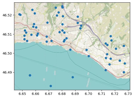
../_images/aaf7dfb089c4d3af6920cba7fa0bb69a00ada468988bd4bfd26a2b800eda5426.png

(C) OpenStreetMap contributors, Tiles style by Humanitarian OpenStreetMap Team hosted by OpenStreetMap France

Mislocated stations#

Before retrieving any time series data, we can filter out some locations just based on their geolocation using the meteora.qc.get_mislocated_stations_method, which will return the list of station ids (index keys in client.stations_gdf) that are considered mislocated. As noted by Meier et al. (2017) (Meier et al., 2017), many Netatmo stations show identical geolocation, which is likely because an inadequate set up “led to automated location assignment based on the IP address of the wireless network” (Napoly et al., 2018) (page 4). Let us plot them in a map:

mislocated_stations = qc.get_mislocated_stations(stations_gdf["geometry"])
ax = stations_gdf.assign(
    label=[
        "mislocated" if i in mislocated_stations else "correct"
        for i in stations_gdf.index
    ]
).plot("label", legend=True)
cx.add_basemap(ax, crs=stations_gdf.crs, attribution="")

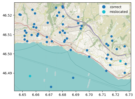
../_images/e65af08c2991b27e13e05cba04c6f592b5ab4a5ca8a3d437f34286b4c79d63da.png

(C) OpenStreetMap contributors, Tiles style by Humanitarian OpenStreetMap Team hosted by OpenStreetMap France

As we can see, some of the mislocated stations, but not all of them, are on Lake Geneva. The other stations on the lake are likely mislocated too and can be filtered out using an ad-hoc method.

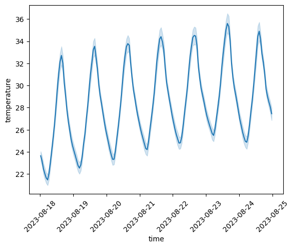
Let us now get a time series of data during a heatwave in August 2023, defined as at least 3 consecutive days with an average temperature over 25$^{\circ}$C (based on the heat level warning definitions by MeteoSwiss):

variables = ["temperature"]
start = "18-08-2023"
end = "25-08-2023"

if use_netatmo_files:
    # query Netatmo data from the API
    long_ts_df = pd.read_csv(
        netatmo_ts_filepath,
        index_col=[settings.STATIONS_ID_COL, settings.TIME_COL],
        parse_dates=True,
    )
    long_ts_df = long_ts_df[variables]
else:
    # fallback to a local file when interactive auth is not possible
    long_ts_df = client.get_ts_df(variables, start, end, scale=scale)

/tmp/ipykernel_1323/542212961.py:7: UserWarning: Could not infer format, so each element will be parsed individually, falling back to `dateutil`. To ensure parsing is consistent and as-expected, please specify a format.
  long_ts_df = pd.read_csv(

We can now plot the time series of CWS observations. Since there are 59 CWS in the study area (number of rows in client.stations_gdf), we can use the seaborn.lineplot function to plot the mean and 95% confidence intervals at each temporal cross-section:

ax = sns.lineplot(long_ts_df.reset_index(), x="time", y="temperature")
ax.tick_params(axis="x", labelrotation=45)

../_images/b923c801084021fb6e9afacd4ccb2c1858e60145acbaaf2829252bf15819e035.png

The get_ts_df method of all Meteora clients returns a long-form time series data frames, multi-indexed by stations (first-level) and time (second-level) and with variables as columns. However, the methods of the qc module expect a wide-form time series data frame instead, where each cell represents the temperature measurement at a given time (index) and station (columns). See the “Data structures” section of the Meteora documentation for more details.

We can use the meteora.utils.long_to_wide function to transform a time series data frame from its long form to its wide form. Let us do that and start by filtering out the mislocated stations:

ts_df = utils.long_to_wide(long_ts_df)
# discard mislocated stations
ts_df = ts_df.drop(columns=mislocated_stations, errors="ignore")

Note that we are using the errors="ignore" keyword argument when discarding stations because some stations in client.stations_gdf may not have data for the requested period and thus may not appear in the time series data frames. The default errors="raise" would instead raise a KeyError.

Unreliable stations#

After discarding the mislocated stations, we can continue with a very simple QC to filter out stations with not enough valid observations during the study period. This is done by the meteora.qc.get_unreliable_stations function, which besides the (wide) time series data frame, accepts an optional unreliable_threshold keyword argument (otherwise the default set in meteora.settings.UNRELIABLE_THRESHOLD is used). Let us thus discard stations that have more than 20% of missing observations for the study period:

unreliable_threshold = 0.2
unreliable_stations = qc.get_unreliable_stations(
    ts_df, unreliable_threshold=unreliable_threshold
)
unreliable_stations

['70:ee:50:27:41:ac', '70:ee:50:90:79:f4']

At any QC step we can use the meteora.qc.comparison_lineplot function to compare the time series of the discarded and kept stations. In this case, since there are only 2 unreliable stations, we will use the individual_discard_lines=True keyword argument (default False) to plot each unreliable station’s line individually rather than plotting the mean plus confidence interval, which would not let us appreciate the periods with non-valid data:

qc.comparison_lineplot(
    ts_df,
    unreliable_stations,
    label_discarded="unreliable",
    label_kept="reliable",
    individual_discard_lines=True,
)

<Axes: xlabel='time', ylabel='temperature'>

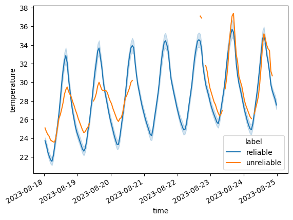
../_images/5d9cad24bdf82b09c220708fc33326afc866c8ba57fc2aefbf6cc0dd22afd807.png

Filtering out unreliable stations should be the first step of the time series-based QC, since otherwise QC functions may return misleading results:

reliable_ts_df = ts_df.drop(columns=unreliable_stations)

Elevation adjustment (optional)#

Due to the atmospheric lapse rate, stations at lower elevations are usually expected to be consistently warmer than its counterparts at higher elevations (except under, e.g., the occurrence of inversion). Therefore, it is possible to adjust for the elevation the time series data frame - otherwise we may find, e.g., that a given station is consistently warmer because of an incorrect set up when in reality the difference is due to the elevation. This can be done using the meteora.qc.elevation_adjustment function, which besides the (wide) time series data frame, accepts an optional atmospheric_lapse_rate keyword argument (otherwise the default set in meteora.settings.ATMOSPHERIC_LAPSE_RATE is used):

atmospheric_lapse_rate = 0.0065  # in C / m
adj_ts_df = qc.elevation_adjustment(
    reliable_ts_df,
    stations_gdf["altitude"],
    atmospheric_lapse_rate=atmospheric_lapse_rate,
)

Let us now plot the difference between the average elevation-adjusted and unadjusted temperature at each station:

ax = stations_gdf.assign(diff=adj_ts_df.mean() - reliable_ts_df.mean()).plot(
    "diff",
    legend=True,
    legend_kwds={
        "label": "$\overline{T_{adj}} - \overline{T} \quad [\circ C]$",
        "shrink": 0.6,
    },
)
cx.add_basemap(ax, crs=stations_gdf.crs, attribution="")
stations_gdf["altitude"].describe()[["mean", "min", "max"]]

<>:5: SyntaxWarning: invalid escape sequence '\o'
<>:5: SyntaxWarning: invalid escape sequence '\o'
/tmp/ipykernel_1323/3365188783.py:5: SyntaxWarning: invalid escape sequence '\o'
  "label": "$\overline{T_{adj}} - \overline{T} \quad [\circ C]$",

mean    504.745763
min     370.000000
max     764.000000
Name: altitude, dtype: float64

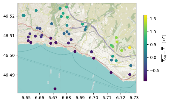
../_images/6e43f024cbde9bc0236f2fcada61ec3dbaf433d3e95ebd3a6b715f2fe1ecdbc1.png

Stations at higher elevations are added about 1.5 $^{\circ}$C whereas the ones at lower elevations are subtracted less than that (because of the smaller elevation difference between the mean and the minimum than between the maximum and the mean).

Oulier stations#

The meteora.qc.get_outlier_stations allows detecting when the measurements of a given station show suspicious deviations from a normal distribution. The function allow three optional keyword arguments, namely low_alpha and high_alpha, which are the respective values for the lower and upper tail that lead to a rejection of the null hypothesis (and that default to meteora.settings.OUTLIER_LOW_ALPHA and meteora.settings.OUTLIER_LOW_ALPHA respectively) as well as station_outlier_threshold, which is the maximum proportion of outlier measurements after which the respective station is flagged as faulty (defaults to meteora.settings.station_outlier_threshold). As noted by Meier et al., (2017) (Meier et al., 2017), one of the main issues with Netatmo data are stations located in non-shaded areas, resulting in radiative errors, which is why the upper tail threshold is by default less permisive than its lower tail counterpart.

We can detect outlier stations separately for the initial data frame with (i) all (but mislocated) stations, (ii) reliable stations and (ii) reliable stations with elevation adjustment:

low_alpha = 0.01
high_alpha = 0.95
station_outlier_threshold = 0.2

for _ts_df, label in zip(
    [ts_df, reliable_ts_df, adj_ts_df], ["raw", "reliable", "elev. adjusted"]
):
    outlier_stations = qc.get_outlier_stations(
        _ts_df,
        low_alpha=low_alpha,
        high_alpha=high_alpha,
        station_outlier_threshold=station_outlier_threshold,
    )
    print(f"n. outlier stations from {label}: {len(outlier_stations)}")
outlier_stations = qc.get_outlier_stations(reliable_ts_df)

n. outlier stations from raw: 3
n. outlier stations from reliable: 3
n. outlier stations from elev. adjusted: 2

As we can see, initially 3 stations would be considered outliers, but after we exclude the unreliable stations, the number drops to 1 (with or without elevation adjustment). This highlights the importance of excluding unreliable stations first, otherwise we may wrongfully assume that the unreliable stations are systematically warmer or colder whereas in fact they likely do not have enough measurements to determine that.

For the reminder of the notebook, let us consider the outlier stations from the unadjusted reliable stations. We can again use the comparison_lineplot method:

qc.comparison_lineplot(
    reliable_ts_df,
    outlier_stations,
    label_discarded="outlier",
    label_kept="non-outlier",
)

<Axes: xlabel='time', ylabel='temperature'>

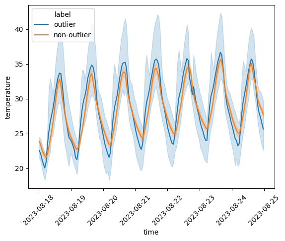
../_images/2483b662d0bf36aa70142e380e46b0bc18d9bf376e64a1f0528afa1e27916cf2.png

Stations labeled as outliers clearly display an amplified temperature variation, especially for the maximum temperatures - in line with the radiative errors suggested by Meier et al. (2017) (Meier et al., 2017).

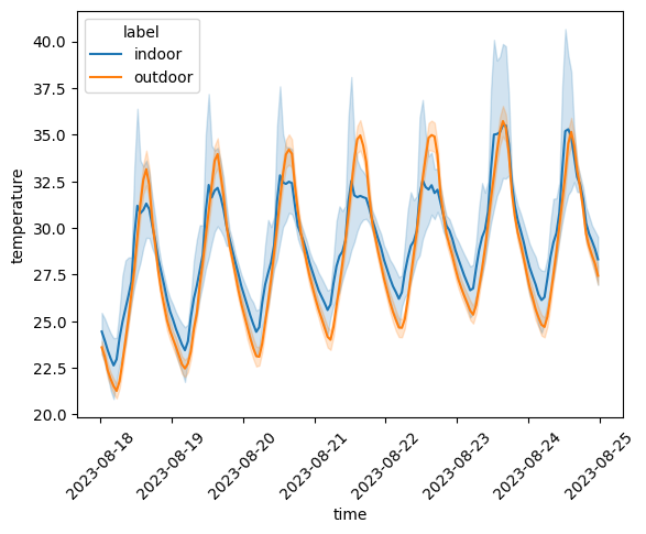
Indoor stations#

Netatmo stations may also be set indoors, in which case their diurnal cycles are assumed to be less correlated to the one from outdoor stations (Napoly et al., 2018). To that end, we can use the meteora.qc.get_indoor_stations function, which accepts an optional keyword argument station_indoor_corr_threshold, so that stations showing Pearson correlation (with the overall station median distribution) lower than the provided value are flagged as indoors (which defaults to meteora.settings.STATION_INDOOR_CORR_THRESHOLD):

station_indoor_corr_threshold = 0.9

indoor_stations = qc.get_indoor_stations(
    reliable_ts_df, station_indoor_corr_threshold=station_indoor_corr_threshold
)
indoor_stations

['70:ee:50:00:71:0a',
 '70:ee:50:00:78:82',
 '70:ee:50:27:66:ba',
 '70:ee:50:28:89:d4',
 '70:ee:50:29:2c:ca',
 '70:ee:50:65:70:a2',
 '70:ee:50:9c:e8:d6']

In this example, 7 stations are considered to be indoors. We can check whether any indoor station is also considered an outlier:

set(indoor_stations).intersection(set(outlier_stations))

{'70:ee:50:28:89:d4'}

which is not the case. We can also plot the time series of temperature measurements for indoor and outdoor stations separately:

qc.comparison_lineplot(
    reliable_ts_df,
    indoor_stations,
    label_discarded="indoor",
    label_kept="outdoor",
)

<Axes: xlabel='time', ylabel='temperature'>

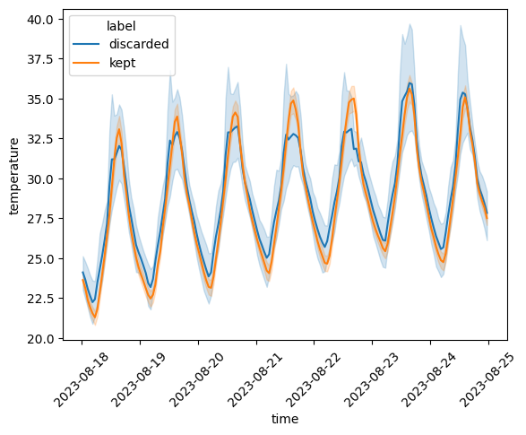
../_images/12367015dce2c9e057756cf6e5e2246ce8d0c6bc0eea7ddaf2d5959332824875.png

To conclude the QC, we can combine all the QC filters and plot the kept and discarded stations:

discarded_stations = list(set(outlier_stations) | set(indoor_stations))
qc.comparison_lineplot(
    reliable_ts_df,
    list(set(outlier_stations) | set(indoor_stations)),
)

<Axes: xlabel='time', ylabel='temperature'>

../_images/e89922743be06b966e27a689f960fc3788a47290f0d57fd35efd23a274ff5f86.png

Comparison with official data#

Finally, we can compare the time series of temperature measurements of the CWS data (before and after QC) with its counterpart from official stations. To that end, we will get the data from Agrometeo and MeteoSwiss:

# official
# need to specify the crs for agrometeo, otherwise it will be epsg:21781
agrometeo_client = clients.AgrometeoClient(region, crs=crs)
meteoswiss_client = clients.MeteoSwissClient(region)

ax = pd.concat(
    [
        stations_gdf.assign(source=label).to_crs(crs)
        for label, stations_gdf in {
            "Netatmo": stations_gdf,
            "Agrometeo": agrometeo_client.stations_gdf,
            "MeteoSwiss": meteoswiss_client.stations_gdf,
        }.items()
    ]
).plot("source", legend=True)
cx.add_basemap(ax, crs=crs, attribution="")

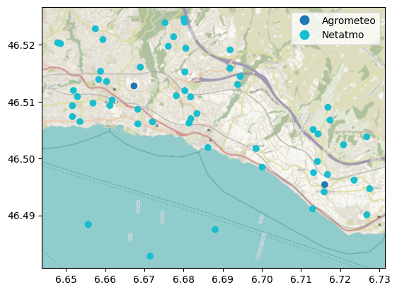
../_images/7329a380995bb138c8e6e6ab17ffae39aa69b86bc46bc9896fdf3a48cdad2519.png

There are only a few official stations in the study area compared with the high spatial density of Netatmo CWS. Let us now get the time series of temperature data for the study period:

# specify hourly `scale` for Agrometeo, otherwise is 10-minutes.
agrometeo_ts_df = agrometeo_client.get_ts_df(variables, start, end, scale="hour")
meteoswiss_ts_df = meteoswiss_client.get_ts_df(variables, start, end)

---------------------------------------------------------------------------
KeyError                                  Traceback (most recent call last)
Cell In[21], line 3
# specify hourly `scale` for Agrometeo, otherwise is 10-minutes.
agrometeo_ts_df = agrometeo_client.get_ts_df(variables, start, end, scale="hour")
----> 3 meteoswiss_ts_df = meteoswiss_client.get_ts_df(variables, start, end)

File ~/checkouts/readthedocs.org/user_builds/meteora/checkouts/latest/meteora/clients/meteoswiss.py:305, in MeteoSwissClient.get_ts_df(self, variables, start, end)
def get_ts_df(
   self,
   variables: VariablesType,
   start: DateTimeType,
   end: DateTimeType,
) -> pd.DataFrame:
   """Get time series data frame.

   Parameters
   (...)    303         at each station (first-level index) for each variable (column).
   """
--> 305     return self._get_ts_df(
       variables=variables,
       start=start,
       end=end,
   )

File ~/checkouts/readthedocs.org/user_builds/meteora/checkouts/latest/meteora/clients/base.py:253, in BaseClient._get_ts_df(self, variables, *args, **kwargs)
ts_df = self._ts_df_from_endpoint(ts_params)
# ACHTUNG: do NOT set the station, time multi-index here because this is already
# done in `_ts_df_from_content` in many cases since it results from groupby,
# stack or pivot operations
   (...)    251 # `variables` argument (e.g., if the user provided variable codes, use
# variable codes in the column names).
--> 253 ts_df = self._rename_variables_cols(ts_df, variable_id_ser)
# apply a generic post-processing function (by default, ensuring numeric dtypes
# and sorting)
ts_df = self._post_process_ts_df(ts_df)

File ~/checkouts/readthedocs.org/user_builds/meteora/checkouts/latest/meteora/clients/base.py:171, in BaseClient._rename_variables_cols(self, ts_df, variable_id_ser)
def _rename_variables_cols(
   self, ts_df: pd.DataFrame, variable_id_ser: pd.Series
) -> pd.DataFrame:
   # TODO: avoid this if the user provided variable codes (in which case the dict
   # maps variable codes to variable codes)?
   # also keep only columns of requested variables
--> 171     return ts_df[variable_id_ser].rename(
       columns={
           variable_id: variable
           for variable, variable_id in variable_id_ser.items()
       }
   )

File ~/checkouts/readthedocs.org/user_builds/meteora/checkouts/latest/.pixi/envs/doc/lib/python3.13/site-packages/pandas/core/frame.py:4384, in DataFrame.__getitem__(self, key)
   if is_iterator(key):
       key = list(key)
-> 4384     indexer = self.columns._get_indexer_strict(key, "columns")[1]
# take() does not accept boolean indexers
if getattr(indexer, "dtype", None) == bool:

File ~/checkouts/readthedocs.org/user_builds/meteora/checkouts/latest/.pixi/envs/doc/lib/python3.13/site-packages/pandas/core/indexes/base.py:6302, in Index._get_indexer_strict(self, key, axis_name)
else:
   keyarr, indexer, new_indexer = self._reindex_non_unique(keyarr)
-> 6302 self._raise_if_missing(keyarr, indexer, axis_name)
keyarr = self.take(indexer)
if isinstance(key, Index):
   # GH 42790 - Preserve name from an Index

File ~/checkouts/readthedocs.org/user_builds/meteora/checkouts/latest/.pixi/envs/doc/lib/python3.13/site-packages/pandas/core/indexes/base.py:6352, in Index._raise_if_missing(self, key, indexer, axis_name)
if nmissing:
   if nmissing == len(indexer):
-> 6352         raise KeyError(f"None of [{key}] are in the [{axis_name}]")
   not_found = list(ensure_index(key)[missing_mask.nonzero()[0]].unique())
   raise KeyError(f"{not_found} not in index")

KeyError: "None of [Index(['tre200s0'], dtype='str')] are in the [columns]"

We can now plot the time series separately. To have more flexibility, we will use the long-form data frames (note that we thus need to exlude the mislocated stations again, which were already excluded from the wide-form data frame but not from the long-form one):

all_discards = list(
    set(discarded_stations) | set(unreliable_stations) | set(mislocated_stations)
)
ax = sns.lineplot(
    pd.concat(
        [
            ts_df.assign(label=label)
            for ts_df, label in zip(
                [
                    long_ts_df.drop(all_discards, errors="ignore"),
                    long_ts_df.loc[discarded_stations],
                    pd.concat([agrometeo_ts_df, meteoswiss_ts_df]),
                ],
                ["CWS (QC)", "CWS (Discarded)", "Official"],
            )
        ]
    )
    .droplevel("station_id")
    .reset_index(),
    x="time",
    y="temperature",
    hue="label",
)
ax.tick_params(axis="x", labelrotation=45)

We can observe how, unlike the discarded CWS, the CWS that pass QC have a very similar trend as the official stations. Although this is beyond the scope of this notebook, note that even after QC, CWS seem to be slightly warmer than the official stations, but this may be due to elevation differences as well as the urban heat island effect.

References#

[1] (1,2,3,4)

Fred Meier, Daniel Fenner, Tom Grassmann, Marco Otto, and Dieter Scherer. Crowdsourcing air temperature from citizen weather stations for urban climate research. Urban Climate, 19:170–191, 2017.

[2]

C. L. Muller, L. Chapman, S. Johnston, C. Kidd, S. Illingworth, G. Foody, and R. R. Leigh. Crowdsourcing for climate and atmospheric sciences: current status and future potential. International Journal of Climatology, 35(11):3185–3203, 2015.

[3] (1,2,3)

Adrien Napoly, Tom Grassmann, Fred Meier, and Daniel Fenner. Development and application of a statistically-based quality control for crowdsourced air temperature data. Frontiers in Earth Science, pages 118, 2018.